Note
This page was generated from Notebooks/flopy3_modpath7_structured_example.ipynb.
Interactive online version: 
Using MODPATH 7 with structured grids
This notebook demonstrates how to create and run example 1a from the MODPATH 7 documentation for MODFLOW-2005 and MODFLOW 6. The notebooks also shows how to create subsets of endpoint output and plot MODPATH results on PlotMapView objects.
[1]:
import sys
import os
from tempfile import TemporaryDirectory

import numpy as np
import matplotlib as mpl
import matplotlib.pyplot as plt

# run installed version of flopy or add local path
try:
    import flopy
except:
    fpth = os.path.abspath(os.path.join("..", ".."))
    sys.path.append(fpth)
    import flopy

    print(sys.version)
print("numpy version: {}".format(np.__version__))
print("matplotlib version: {}".format(mpl.__version__))
print("flopy version: {}".format(flopy.__version__))

# temporary directory
temp_dir = TemporaryDirectory()
workspace = temp_dir.name
numpy version: 1.24.3
matplotlib version: 3.7.1
flopy version: 3.3.7
Flow model data
[2]:
nper, nstp, perlen, tsmult = 1, 1, 1.0, 1.0
nlay, nrow, ncol = 3, 21, 20
delr = delc = 500.0
top = 400.0
botm = [220.0, 200.0, 0.0]
laytyp = [1, 0, 0]
kh = [50.0, 0.01, 200.0]
kv = [10.0, 0.01, 20.0]
wel_loc = (2, 10, 9)
wel_q = -150000.0
rch = 0.005
riv_h = 320.0
riv_z = 317.0
riv_c = 1.0e5
MODPATH 7 data
[3]:
# MODPATH zones
zone3 = np.ones((nrow, ncol), dtype=np.int32)
zone3[wel_loc[1:]] = 2
zones = [1, 1, zone3]

# create particles
# particle group 1
plocs = []
pids = []
for idx in range(nrow):
    plocs.append((0, idx, 2))
    pids.append(idx)
part0 = flopy.modpath.ParticleData(
    plocs, drape=0, structured=True, particleids=pids
)
pg0 = flopy.modpath.ParticleGroup(
    particlegroupname="PG1", particledata=part0, filename="ex01a.pg1.sloc"
)

# particle group 2
v = [(2, 0, 0), (0, 20, 0)]
part1 = flopy.modpath.ParticleData(
    v, drape=1, structured=True, particleids=[1000, 1001]
)
pg1 = flopy.modpath.ParticleGroup(
    particlegroupname="PG2", particledata=part1, filename="ex01a.pg2.sloc"
)

locsa = [[0, 0, 0, 0, nrow - 1, ncol - 1], [1, 0, 0, 1, nrow - 1, ncol - 1]]
locsb = [[2, 0, 0, 2, nrow - 1, ncol - 1]]
sd = flopy.modpath.CellDataType(
    drape=0, columncelldivisions=1, rowcelldivisions=1, layercelldivisions=1
)
p = flopy.modpath.LRCParticleData(
    subdivisiondata=[sd, sd], lrcregions=[locsa, locsb]
)
pg2 = flopy.modpath.ParticleGroupLRCTemplate(
    particlegroupname="PG3", particledata=p, filename="ex01a.pg3.sloc"
)

particlegroups = [pg2]

# default iface for MODFLOW-2005 and MODFLOW 6
defaultiface = {"RECHARGE": 6, "ET": 6}
defaultiface6 = {"RCH": 6, "EVT": 6}
MODPATH 7 using MODFLOW-2005
Create and run MODFLOW-2005
[4]:
ws = os.path.join(workspace, "mp7_ex1_mf2005_dis")
nm = "ex01_mf2005"
exe_name = "mf2005"
iu_cbc = 130
m = flopy.modflow.Modflow(nm, model_ws=ws, exe_name=exe_name)
flopy.modflow.ModflowDis(
    m,
    nlay=nlay,
    nrow=nrow,
    ncol=ncol,
    nper=nper,
    itmuni=4,
    lenuni=2,
    perlen=perlen,
    nstp=nstp,
    tsmult=tsmult,
    steady=True,
    delr=delr,
    delc=delc,
    top=top,
    botm=botm,
)
flopy.modflow.ModflowLpf(
    m, ipakcb=iu_cbc, laytyp=laytyp, hk=kh, vka=kv, constantcv=True
)
flopy.modflow.ModflowBas(m, ibound=1, strt=top)
# recharge
flopy.modflow.ModflowRch(m, ipakcb=iu_cbc, rech=rch)
# wel
wd = [i for i in wel_loc] + [wel_q]
flopy.modflow.ModflowWel(m, ipakcb=iu_cbc, stress_period_data={0: wd})
# river
rd = []
for i in range(nrow):
    rd.append([0, i, ncol - 1, riv_h, riv_c, riv_z])
flopy.modflow.ModflowRiv(m, ipakcb=iu_cbc, stress_period_data={0: rd})
# output control
flopy.modflow.ModflowOc(
    m, stress_period_data={(0, 0): ["save head", "save budget", "print head"]}
)
flopy.modflow.ModflowPcg(m, hclose=1e-6, rclose=1e-6)

m.write_input()
success, buff = m.run_model(silent=True, report=True)
assert success, "mf2005 model did not run"
for line in buff:
    print(line)
                                  MODFLOW-2005
    U.S. GEOLOGICAL SURVEY MODULAR FINITE-DIFFERENCE GROUND-WATER FLOW MODEL
                             Version 1.12.00 2/3/2017

 Using NAME file: ex01_mf2005.nam
 Run start date and time (yyyy/mm/dd hh:mm:ss): 2023/05/04 16:06:03

 Solving:  Stress period:     1    Time step:     1    Ground-Water Flow Eqn.
 Run end date and time (yyyy/mm/dd hh:mm:ss): 2023/05/04 16:06:03
 Elapsed run time:  0.015 Seconds

  Normal termination of simulation
Create and run MODPATH 7
[5]:
# create modpath files
exe_name = "mp7"
mp = flopy.modpath.Modpath7(
    modelname=nm + "_mp", flowmodel=m, exe_name=exe_name, model_ws=ws
)
mpbas = flopy.modpath.Modpath7Bas(mp, porosity=0.1, defaultiface=defaultiface)
mpsim = flopy.modpath.Modpath7Sim(
    mp,
    simulationtype="combined",
    trackingdirection="forward",
    weaksinkoption="pass_through",
    weaksourceoption="pass_through",
    budgetoutputoption="summary",
    budgetcellnumbers=[1049, 1259],
    traceparticledata=[1, 1000],
    referencetime=[0, 0, 0.0],
    stoptimeoption="extend",
    timepointdata=[500, 1000.0],
    zonedataoption="on",
    zones=zones,
    particlegroups=particlegroups,
)

# write modpath datasets
mp.write_input()

# run modpath
success, buff = mp.run_model(silent=True, report=True)
assert success, "mp7 failed to run"
for line in buff:
    print(line)
MODPATH Version 7.2.001
Program compiled Apr 12 2023 19:05:18 with IFORT compiler (ver. 20.21.7)


Run particle tracking simulation ...
Processing Time Step     1 Period     1.  Time =  1.00000E+00  Steady-state flow

Particle Summary:
         0 particles are pending release.
         0 particles remain active.
         0 particles terminated at boundary faces.
         0 particles terminated at weak sink cells.
         0 particles terminated at weak source cells.
      1260 particles terminated at strong source/sink cells.
         0 particles terminated in cells with a specified zone number.
         0 particles were stranded in inactive or dry cells.
         0 particles were unreleased.
         0 particles have an unknown status.

Normal termination.
Load MODPATH 7 output
Get locations to extract pathline data
[6]:
nodew = m.dis.get_node([wel_loc])
riv_locs = flopy.utils.ra_slice(m.riv.stress_period_data[0], ["k", "i", "j"])
nodesr = m.dis.get_node(riv_locs.tolist())
Pathline data
[7]:
fpth = os.path.join(ws, nm + "_mp.mppth")
p = flopy.utils.PathlineFile(fpth)
pw0 = p.get_destination_pathline_data(nodew, to_recarray=True)
pr0 = p.get_destination_pathline_data(nodesr, to_recarray=True)
Endpoint data
Get particles that terminate in the well
[8]:
fpth = os.path.join(ws, nm + "_mp.mpend")
e = flopy.utils.EndpointFile(fpth)
well_epd = e.get_destination_endpoint_data(dest_cells=nodew)
well_epd.shape
[8]:
(564,)
Get particles that terminate in the river boundaries
[9]:
riv_epd = e.get_destination_endpoint_data(dest_cells=nodesr)
riv_epd.shape
[9]:
(696,)
Merge the particles that end in the well and the river boundaries.
[10]:
epd0 = np.concatenate((well_epd, riv_epd))
epd0.shape
[10]:
(1260,)
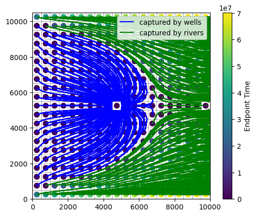
Plot MODPATH 7 output
[11]:
mm = flopy.plot.PlotMapView(model=m)
mm.plot_grid(lw=0.5)
mm.plot_pathline(pw0, layer="all", colors="blue", label="captured by wells")
mm.plot_pathline(pr0, layer="all", colors="green", label="captured by rivers")
mm.plot_endpoint(epd0, direction="starting", colorbar=True)
mm.ax.legend();

MODPATH 7 using MODFLOW 6
Create and run MODFLOW 6
[12]:
ws = os.path.join(workspace, "mp7_ex1_mf6_dis")
nm = "ex01_mf6"
exe_name = "mf6"

# Create the Flopy simulation object
sim = flopy.mf6.MFSimulation(
    sim_name=nm, exe_name="mf6", version="mf6", sim_ws=ws
)

# Create the Flopy temporal discretization object
pd = (perlen, nstp, tsmult)
tdis = flopy.mf6.modflow.mftdis.ModflowTdis(
    sim, pname="tdis", time_units="DAYS", nper=nper, perioddata=[pd]
)

# Create the Flopy groundwater flow (gwf) model object
model_nam_file = "{}.nam".format(nm)
gwf = flopy.mf6.ModflowGwf(
    sim, modelname=nm, model_nam_file=model_nam_file, save_flows=True
)

# Create the Flopy iterative model solver (ims) Package object
ims = flopy.mf6.modflow.mfims.ModflowIms(
    sim,
    pname="ims",
    complexity="SIMPLE",
    outer_dvclose=1e-6,
    inner_dvclose=1e-6,
    rcloserecord=1e-6,
)

# create gwf file
dis = flopy.mf6.modflow.mfgwfdis.ModflowGwfdis(
    gwf,
    pname="dis",
    nlay=nlay,
    nrow=nrow,
    ncol=ncol,
    length_units="FEET",
    delr=delr,
    delc=delc,
    top=top,
    botm=botm,
)
# Create the initial conditions package
ic = flopy.mf6.modflow.mfgwfic.ModflowGwfic(gwf, pname="ic", strt=top)

# Create the node property flow package
npf = flopy.mf6.modflow.mfgwfnpf.ModflowGwfnpf(
    gwf, pname="npf", icelltype=laytyp, k=kh, k33=kv
)


# recharge
flopy.mf6.modflow.mfgwfrcha.ModflowGwfrcha(gwf, recharge=rch)
# wel
wd = [(wel_loc, wel_q)]
flopy.mf6.modflow.mfgwfwel.ModflowGwfwel(
    gwf, maxbound=1, stress_period_data={0: wd}
)
# river
rd = []
for i in range(nrow):
    rd.append([(0, i, ncol - 1), riv_h, riv_c, riv_z])
flopy.mf6.modflow.mfgwfriv.ModflowGwfriv(gwf, stress_period_data={0: rd})
# Create the output control package
headfile = "{}.hds".format(nm)
head_record = [headfile]
budgetfile = "{}.cbb".format(nm)
budget_record = [budgetfile]
saverecord = [("HEAD", "ALL"), ("BUDGET", "ALL")]
oc = flopy.mf6.modflow.mfgwfoc.ModflowGwfoc(
    gwf,
    pname="oc",
    saverecord=saverecord,
    head_filerecord=head_record,
    budget_filerecord=budget_record,
)

# Write the datasets
sim.write_simulation()
# Run the simulation
success, buff = sim.run_simulation(silent=True, report=True)
assert success, "mf6 model did not run"
for line in buff:
    print(line)
writing simulation...
  writing simulation name file...
  writing simulation tdis package...
  writing solution package ims...
  writing model ex01_mf6...
    writing model name file...
    writing package dis...
    writing package ic...
    writing package npf...
    writing package rcha_0...
    writing package wel_0...
    writing package riv_0...
INFORMATION: maxbound in ('gwf6', 'riv', 'dimensions') changed to 21 based on size of stress_period_data
    writing package oc...
                                   MODFLOW 6
                U.S. GEOLOGICAL SURVEY MODULAR HYDROLOGIC MODEL
                        VERSION 6.4.1 Release 12/09/2022

   MODFLOW 6 compiled Apr 12 2023 19:02:29 with Intel(R) Fortran Intel(R) 64
   Compiler Classic for applications running on Intel(R) 64, Version 2021.7.0
                             Build 20220726_000000

This software has been approved for release by the U.S. Geological
Survey (USGS). Although the software has been subjected to rigorous
review, the USGS reserves the right to update the software as needed
pursuant to further analysis and review. No warranty, expressed or
implied, is made by the USGS or the U.S. Government as to the
functionality of the software and related material nor shall the
fact of release constitute any such warranty. Furthermore, the
software is released on condition that neither the USGS nor the U.S.
Government shall be held liable for any damages resulting from its
authorized or unauthorized use. Also refer to the USGS Water
Resources Software User Rights Notice for complete use, copyright,
and distribution information.


 Run start date and time (yyyy/mm/dd hh:mm:ss): 2023/05/04 16:06:16

 Writing simulation list file: mfsim.lst
 Using Simulation name file: mfsim.nam

    Solving:  Stress period:     1    Time step:     1

 Run end date and time (yyyy/mm/dd hh:mm:ss): 2023/05/04 16:06:16
 Elapsed run time:  0.036 Seconds

 Normal termination of simulation.
Create and run MODPATH 7
[13]:
# create modpath files
exe_name = "mp7"
mp = flopy.modpath.Modpath7(
    modelname=nm + "_mp", flowmodel=gwf, exe_name=exe_name, model_ws=ws
)
mpbas = flopy.modpath.Modpath7Bas(mp, porosity=0.1, defaultiface=defaultiface6)
mpsim = flopy.modpath.Modpath7Sim(
    mp,
    simulationtype="combined",
    trackingdirection="forward",
    weaksinkoption="pass_through",
    weaksourceoption="pass_through",
    budgetoutputoption="summary",
    budgetcellnumbers=[1049, 1259],
    traceparticledata=[1, 1000],
    referencetime=[0, 0, 0.0],
    stoptimeoption="extend",
    timepointdata=[500, 1000.0],
    zonedataoption="on",
    zones=zones,
    particlegroups=particlegroups,
)

# write modpath datasets
mp.write_input()

# run modpath
success, buff = mp.run_model(silent=True, report=True)
assert success, "mp7 failed to run"
for line in buff:
    print(line)
MODPATH Version 7.2.001
Program compiled Apr 12 2023 19:05:18 with IFORT compiler (ver. 20.21.7)


Run particle tracking simulation ...
Processing Time Step     1 Period     1.  Time =  1.00000E+00  Steady-state flow

Particle Summary:
         0 particles are pending release.
         0 particles remain active.
         0 particles terminated at boundary faces.
         0 particles terminated at weak sink cells.
         0 particles terminated at weak source cells.
      1260 particles terminated at strong source/sink cells.
         0 particles terminated in cells with a specified zone number.
         0 particles were stranded in inactive or dry cells.
         0 particles were unreleased.
         0 particles have an unknown status.

Normal termination.
Load MODPATH 7 output
Pathline data
[14]:
fpth = os.path.join(ws, nm + "_mp.mppth")
p = flopy.utils.PathlineFile(fpth)
pw1 = p.get_destination_pathline_data(nodew, to_recarray=True)
pr1 = p.get_destination_pathline_data(nodesr, to_recarray=True)
Endpoint data
Get particles that terminate in the well
[15]:
fpth = os.path.join(ws, nm + "_mp.mpend")
e = flopy.utils.EndpointFile(fpth)
well_epd = e.get_destination_endpoint_data(dest_cells=nodew)
Get particles that terminate in the river boundaries
[16]:
riv_epd = e.get_destination_endpoint_data(dest_cells=nodesr)
Merge the particles that end in the well and the river boundaries.
[17]:
epd1 = np.concatenate((well_epd, riv_epd))
Plot MODPATH 7 output
[18]:
mm = flopy.plot.PlotMapView(model=gwf)
mm.plot_grid(lw=0.5)
mm.plot_pathline(pw1, layer="all", colors="blue", label="captured by wells")
mm.plot_pathline(pr1, layer="all", colors="green", label="captured by rivers")
mm.plot_endpoint(epd1, direction="starting", colorbar=True)
mm.ax.legend();
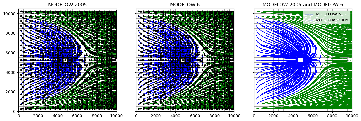
Compare MODPATH results
Compare MODPATH results for MODFLOW-2005 and MODFLOW 6. Also show pathline points every 5th point.
[19]:
f, axes = plt.subplots(ncols=3, nrows=1, sharey=True, figsize=(15, 10))
axes = axes.flatten()
ax = axes[0]
ax.set_aspect("equal")
mm = flopy.plot.PlotMapView(model=m, ax=ax)
mm.plot_grid(lw=0.5)
mm.plot_pathline(
    pw0,
    layer="all",
    colors="blue",
    lw=1,
    marker="o",
    markercolor="black",
    markersize=3,
    markerevery=5,
)
mm.plot_pathline(
    pr0,
    layer="all",
    colors="green",
    lw=1,
    marker="o",
    markercolor="black",
    markersize=3,
    markerevery=5,
)
ax.set_title("MODFLOW-2005")

ax = axes[1]
ax.set_aspect("equal")
mm = flopy.plot.PlotMapView(model=gwf, ax=ax)
mm.plot_grid(lw=0.5)
mm.plot_pathline(
    pw1,
    layer="all",
    colors="blue",
    lw=1,
    marker="o",
    markercolor="black",
    markersize=3,
    markerevery=5,
)
mm.plot_pathline(
    pr1,
    layer="all",
    colors="green",
    lw=1,
    marker="o",
    markercolor="black",
    markersize=3,
    markerevery=5,
)
ax.set_title("MODFLOW 6")


ax = axes[2]
ax.set_aspect("equal")
mm = flopy.plot.PlotMapView(model=m, ax=ax)
mm.plot_grid(lw=0.5)
mm.plot_pathline(pw1, layer="all", colors="blue", lw=1, label="MODFLOW 6")
mm.plot_pathline(
    pw0, layer="all", colors="blue", lw=1, linestyle=":", label="MODFLOW-2005"
)
mm.plot_pathline(pr1, layer="all", colors="green", lw=1, label="_none")
mm.plot_pathline(
    pr0, layer="all", colors="green", lw=1, linestyle=":", label="_none"
)
ax.legend()
ax.set_title("MODFLOW 2005 and MODFLOW 6");