Demo of modflow-obs
This page demonstrates some of the core features of modflow-obs. Specifically:
creation of ‘base’ head and stream flow observations from time series, including
in-tandem processing of observation data and MODFLOW output
automatic spatial and temporal alignment of grid-independent ‘observed’ values and model outputs
creation of instruction files
creating of derivative observations from the base observations, including
sequential temporal changes in observation values at a site
time series of displacement from a reference observation at a site
time series of differences between observed values at two sites
[1]:
from pathlib import Path
import pandas as pd
import matplotlib.pyplot as plt
Inputs
Input and output paths
[2]:
data_path = Path('../mfobs/tests/data/shellmound/')

output_folder = Path('output')
output_folder.mkdir(exist_ok=True)  # make the output folder if it doesn't exist
Model grid definition
For now, we are assuming a uniform structured grid, and using the Affine Package to do this, but this capability could be expanded to support any model grid type, for example by implementing something similar to the model grid object in Flopy.
[3]:
from affine import Affine

# model grid offset and spacing
lower_left_x = 500955.
lower_left_y = 1205285.
# grid spacing along a row, column
delr, delc = 1000., 1000.
modelgrid_transform = Affine(delr, 0., lower_left_x,
                             0., delc, lower_left_y)
model time discretization
read table of stress period information created by modflow-setup
[4]:
perioddata = pd.read_csv(data_path / 'tables/stress_period_data.csv')
perioddata.head()
[4]:
| start_datetime | end_datetime | time | per | perlen | nstp | tsmult | steady | |
|---|---|---|---|---|---|---|---|---|
| 0 | 1998-04-01 | 1998-04-01 | 1.0 | 0 | 1.0 | 1 | 1.0 | True |
| 1 | 1998-04-01 | 2007-03-31 | 3288.0 | 1 | 3287.0 | 10 | 1.5 | False |
| 2 | 2007-04-01 | 2007-09-30 | 3471.0 | 2 | 183.0 | 5 | 1.5 | False |
| 3 | 2007-10-01 | 2008-03-31 | 3654.0 | 3 | 183.0 | 5 | 1.5 | False |
| 4 | 2008-04-01 | 2008-09-30 | 3837.0 | 4 | 183.0 | 5 | 1.5 | False |
alternatively, get the stress period information from the TDIS and STO files
[5]:
from mfobs.modflow import get_perioddata

perioddata = get_perioddata(data_path / 'mfsim.tdis', data_path / 'shellmound.sto')
perioddata.head()
[5]:
| start_datetime | end_datetime | time | per | perlen | nstp | tsmult | steady | |
|---|---|---|---|---|---|---|---|---|
| 0 | 1998-04-01 | 1998-04-01 | 1.0 | 0 | 1.0 | 1 | 1.0 | True |
| 1 | 1998-04-01 | 2007-03-31 | 3288.0 | 1 | 3287.0 | 10 | 1.5 | False |
| 2 | 2007-04-01 | 2007-09-30 | 3471.0 | 2 | 183.0 | 5 | 1.5 | False |
| 3 | 2007-10-01 | 2008-03-31 | 3654.0 | 3 | 183.0 | 5 | 1.5 | False |
| 4 | 2008-04-01 | 2008-09-30 | 3837.0 | 4 | 183.0 | 5 | 1.5 | False |
The above “period_data” table has start/end datetimes in MODFLOW time, but often we want a steady-state period to effectively represent a different time period. Define start and end dates that bracket the time period represented by steady-state period 0:
[6]:
steady_state_period_start = '2008-04-01'
steady_state_period_end = '2008-9-30'
model property information for T-weighted averaging
[7]:
top_array = data_path / 'external/top.dat'
botm_arrays = [data_path / 'external/botm{}.dat'.format(i)
               for i in range(13)]
hk_arrays = [data_path / 'external/k{}.dat'.format(i)
             for i in range(13)]
head observation data
We start with some grid-independent head observation data that already has
been culled to model area, reprojected to the model coordinate references system (real-world x, y locations in UTM or Albers, for example), converted to model units, etc.
open interval information (screen top and bottom elevations)
a column of unique identifiers for each site, which link the site information with time series
prelimary groupings based on location (optional)
The observation data may or may not be broken into a data table with time series, and a metadata table with site information.
The metadata (site info):
[8]:
head_obs_info = pd.read_csv(data_path / 'tables/preprocessed_head_obs_info.csv')
head_obs_info.head()
[8]:
| head | head_std | last_head | n | aqfr_cd | nat_aqfr_cd | screen_botm | screen_top | well_depth | well_el | ... | end_dt | site_no | x | y | well_botm | category | orig_scbot | orig_sctop | obsprefix | group | |
|---|---|---|---|---|---|---|---|---|---|---|---|---|---|---|---|---|---|---|---|---|---|
| 0 | 32.00 | NaN | 32.00 | 1.0 | 112MRVA | N100MSRVVL | NaN | NaN | NaN | 39.05 | ... | 2018-10-01 | USGS:333034090150501 | 530104.14 | 1176208.54 | NaN | 4 | NaN | NaN | USGS:333034090150501 | heads |
| 1 | 26.21 | NaN | 26.21 | 1.0 | 112MRVA | N100MSRVVL | -3.35 | 14.94 | 136.0 | 38.10 | ... | 2006-09-01 | USGS:333040090200601 | 522383.51 | 1175944.23 | -97.90 | 3 | -3.35 | 14.94 | USGS:333040090200601 | heads |
| 2 | 33.15 | 0.0 | 33.15 | 1.6 | 112MRVA | N100MSRVVL | -69.38 | -57.18 | 109.0 | 39.62 | ... | 2002-04-01 | USGS:333050090153001 | 529954.56 | 1176430.50 | -69.38 | 2 | NaN | NaN | USGS:333050090153001 | heads |
| 3 | 20.73 | NaN | 20.73 | 1.0 | 112MRVA | N100MSRVVL | -1.52 | 10.67 | 125.0 | 36.58 | ... | 2002-06-01 | USGS:333113090232001 | 517359.53 | 1176671.36 | -88.42 | 3 | -1.52 | 10.67 | USGS:333113090232001 | heads |
| 4 | 22.83 | NaN | 22.83 | 1.0 | 112MRVA | N100MSRVVL | NaN | NaN | NaN | 37.19 | ... | 2000-10-01 | USGS:333113090244701 | 515142.49 | 1176527.26 | NaN | 4 | NaN | NaN | USGS:333113090244701 | heads |
5 rows × 23 columns
Time series of head at the locations in the metadata:
[9]:
head_obs = pd.read_csv(data_path / 'tables/preprocessed_head_obs.csv')
head_obs.head()
[9]:
| site_no | datetime | head | last_head | head_std | n | obsprefix | |
|---|---|---|---|---|---|---|---|
| 0 | USGS:333034090150501 | 1999-04-01 | 32.37 | 32.37 | NaN | 1 | USGS:333034090150501 |
| 1 | USGS:333034090150501 | 2000-10-01 | 31.54 | 31.54 | NaN | 1 | USGS:333034090150501 |
| 2 | USGS:333034090150501 | 2001-04-01 | 32.60 | 32.60 | NaN | 1 | USGS:333034090150501 |
| 3 | USGS:333034090150501 | 2001-10-01 | 31.96 | 31.96 | NaN | 1 | USGS:333034090150501 |
| 4 | USGS:333034090150501 | 2002-04-01 | 33.35 | 33.35 | NaN | 1 | USGS:333034090150501 |
streamflow observations
Flux observation inputs are similar to heads, except the metadata aren’t needed
only a site number, datetime, and values column are required
Note: site numbers are handled as strings. Site numbers with leading zeros (such as those for many USGS gages) must be specified as strings when read by pandas, otherwise they will be cast to integers by default, and not match the MODFLOW observation names
[10]:
flux_obs = pd.read_csv(data_path / 'tables/processed_flow_obs.csv', dtype={'site_no': object})
flux_obs.head()
[10]:
| site_no | datetime | category | est_qtotal_m3d | est_qbase_m3d | meas_qtotal_m3d | meas_qbase_m3d | obsval | |
|---|---|---|---|---|---|---|---|---|
| 0 | 07281600 | 2008-01-01 | measured | NaN | NaN | 10215000.0 | 6403120.0 | 6403120.0 |
| 1 | 07281600 | 2008-02-01 | measured | NaN | NaN | 15611700.0 | 5332650.0 | 5332650.0 |
| 2 | 07281600 | 2008-03-01 | measured | NaN | NaN | 20682200.0 | 15022400.0 | 15022400.0 |
| 3 | 07281600 | 2008-04-01 | measured | NaN | NaN | 24353200.0 | 12339100.0 | 12339100.0 |
| 4 | 07281600 | 2008-05-01 | measured | NaN | NaN | 22076000.0 | 13931500.0 | 13931500.0 |
MODFLOW-6 observation input
the MODFLOW observation names (representing sites) must match those in the
obsprefixcolumn of the preprocessed head data abovea key feature of Modflow-obs is computation of simulated heads from transmissivity-weighted averages of the head values simulated for the layers that intersect each well open interval. To take advantage of this feature, for each location (site), a MODFLOW observation must be entered for each layer.
Modflow-setup can create MODFLOW-6 observation input (with an observation in each layer) automatically, using the locations and
obsprefixesin the above metadata file
[11]:
headobs_input_file = data_path / 'shellmound.obs'

with open(headobs_input_file) as src:
    print(src.read()[:500])
BEGIN options
  DIGITS  10
  PRINT_INPUT
END options

BEGIN continuous  FILEOUT  shellmound.head.obs
  usgs:333145090261901  HEAD  1 28 12
  usgs:333145090261901  HEAD  2 28 12
  usgs:333145090261901  HEAD  3 28 12
  usgs:333145090261901  HEAD  4 28 12
  usgs:333145090261901  HEAD  5 28 12
  usgs:333145090261901  HEAD  6 28 12
  usgs:333145090261901  HEAD  7 28 12
  usgs:333145090261901  HEAD  8 28 12
  usgs:333145090261901  HEAD  9 28 12
  usgs:333145090261901  HEAD  10 28 12
  usgs:33314509026
flux observation in input to MODFLOW is not needed by modflow-obs because there aren’t layers to sort out, but like head observations, the site identifiers supplied to MODFLOW must match those in the observation data file above
MODFLOW-6 observation output
simulated values at observation locations are returned in a csv file with model timesteps along the row axis, and individual observation locations (1 per layer) along the column axis
[12]:
headobs_output_file = data_path / 'shellmound.head.obs'
with open(headobs_output_file) as src:
    print('\n'.join([l[:100] for l in src.readlines()[:2]]))
time,USGS:333145090261901,USGS:333145090261901,USGS:333145090261901,USGS:333145090261901,USGS:333145
1.000000000000,29.61748720,29.62154020,29.62504962,29.62677031,29.62761331,29.62882679,29.63409325,2
SFR package observations are similar
[13]:
fluxobs_output_file = data_path / 'shellmound.sfr.obs.output.csv'

with open(fluxobs_output_file) as src:
    print(''.join([l for l in src.readlines()[:4]]))
time,07288280,07288580,07288500,07281600
1,0,-1805.6,0,-8.203e+06
30.0038,0,-901.46,0,-8.2845e+06
73.5094,0,0,0,-8.2622e+06
Create a base set of head observations
reads head observation data and model output and matches values
by location using the
obsprefixnamesin time by averaging observed values to the model stress period
optionally, a model stress period can be labeled as steady-state (
label_period_as_steady_state), representing average conditions over a time period bracked by asteady_state_period_startandsteady_state_period_end. In this case, the simulated values for the labeled stress period are matched to average values for the steady-state time period.
the model output are assumed to include all layers at each observation location; observation names in the model output are assumed to correspond to
obsprefixes in the head observation dataobservation layer can be specified explicitly via an
observed_values_layer_colin the head observation data, or, the simulated values can be averaged vertically with transmissivity-based weighting (observed_values_layer_col=None). In the latter case, model property arrays (hk_arrays,top_array,botm_arrays) must be supplied. At observation sites without open interval information, all model layers are included in the transmissivity-weighted averaging.observation names to match observed values to their simulated equivalents are constructed in the format of
<obsprefix>_<date suffix>, where obsprefix is a site identifier taken from theobserved_values_site_id_colinobserved_values_file, and the date suffix is controlled by theobsnme_date_suffix_formatparameter (default of'%Y%m'). Steady-state observations are assigned a suffix of'ss'.simulated and observed values are written to columns formatted with
sim_orobs_<variable_name>
[14]:
from mfobs.heads import get_head_obs

base_obs = get_head_obs(perioddata,
                        modelgrid_transform=modelgrid_transform,
                        model_output_file=headobs_output_file,
                        observed_values_file=head_obs,
                        gwf_obs_input_file=headobs_input_file,
                        observed_values_metadata_file=head_obs_info,
                        observed_values_site_id_col='obsprefix',  # default
                        observed_values_datetime_col='datetime',  # default
                        observed_values_x_col='x',  # default
                        observed_values_y_col='y',  # default
                        observed_values_screen_top_col='screen_top',  # default
                        observed_values_screen_botm_col='screen_botm',  # default
                        observed_values_obsval_col='head',
                        hk_arrays=hk_arrays,
                        top_array=top_array,
                        botm_arrays=botm_arrays,
                        label_period_as_steady_state=0,
                        steady_state_period_start=steady_state_period_start,
                        steady_state_period_end=steady_state_period_end,
                        write_ins=True,
                        outfile=output_folder / 'processed_head_obs.dat'
                        )
base_obs.head()
reading model output from ../mfobs/tests/data/shellmound/shellmound.head.obs...
took 0.01s

Dropping 191 sites with no information
/home/runner/work/modflow-obs/modflow-obs/mfobs/heads.py:653: RuntimeWarning: invalid value encountered in divide
  in_model_frac = (in_model_len / screen_len)
/home/runner/work/modflow-obs/modflow-obs/mfobs/heads.py:685: RuntimeWarning: invalid value encountered in divide
  Tr_frac = T / T.sum(axis=0)
/home/runner/work/modflow-obs/modflow-obs/mfobs/heads.py:653: RuntimeWarning: invalid value encountered in divide
  in_model_frac = (in_model_len / screen_len)
/home/runner/work/modflow-obs/modflow-obs/mfobs/heads.py:685: RuntimeWarning: invalid value encountered in divide
  Tr_frac = T / T.sum(axis=0)
/home/runner/work/modflow-obs/modflow-obs/mfobs/heads.py:653: RuntimeWarning: invalid value encountered in divide
  in_model_frac = (in_model_len / screen_len)
/home/runner/work/modflow-obs/modflow-obs/mfobs/heads.py:685: RuntimeWarning: invalid value encountered in divide
  Tr_frac = T / T.sum(axis=0)
/home/runner/work/modflow-obs/modflow-obs/mfobs/heads.py:653: RuntimeWarning: invalid value encountered in divide
  in_model_frac = (in_model_len / screen_len)
/home/runner/work/modflow-obs/modflow-obs/mfobs/heads.py:685: RuntimeWarning: invalid value encountered in divide
  Tr_frac = T / T.sum(axis=0)
/home/runner/work/modflow-obs/modflow-obs/mfobs/heads.py:653: RuntimeWarning: invalid value encountered in divide
  in_model_frac = (in_model_len / screen_len)
/home/runner/work/modflow-obs/modflow-obs/mfobs/heads.py:685: RuntimeWarning: invalid value encountered in divide
  Tr_frac = T / T.sum(axis=0)
/home/runner/work/modflow-obs/modflow-obs/mfobs/heads.py:653: RuntimeWarning: invalid value encountered in divide
  in_model_frac = (in_model_len / screen_len)
/home/runner/work/modflow-obs/modflow-obs/mfobs/heads.py:685: RuntimeWarning: invalid value encountered in divide
  Tr_frac = T / T.sum(axis=0)
/home/runner/work/modflow-obs/modflow-obs/mfobs/heads.py:653: RuntimeWarning: invalid value encountered in divide
  in_model_frac = (in_model_len / screen_len)
/home/runner/work/modflow-obs/modflow-obs/mfobs/heads.py:685: RuntimeWarning: invalid value encountered in divide
  Tr_frac = T / T.sum(axis=0)
/home/runner/work/modflow-obs/modflow-obs/mfobs/heads.py:653: RuntimeWarning: invalid value encountered in divide
  in_model_frac = (in_model_len / screen_len)
/home/runner/work/modflow-obs/modflow-obs/mfobs/heads.py:685: RuntimeWarning: invalid value encountered in divide
  Tr_frac = T / T.sum(axis=0)
/home/runner/work/modflow-obs/modflow-obs/mfobs/heads.py:578: UserWarning: Stress period 8: No observations between start and end dates of 2010-04-01 and 2010-09-30!
  warnings.warn(('Stress period {}: No observations between start and '
/home/runner/work/modflow-obs/modflow-obs/mfobs/heads.py:653: RuntimeWarning: invalid value encountered in divide
  in_model_frac = (in_model_len / screen_len)
/home/runner/work/modflow-obs/modflow-obs/mfobs/heads.py:685: RuntimeWarning: invalid value encountered in divide
  Tr_frac = T / T.sum(axis=0)
/home/runner/work/modflow-obs/modflow-obs/mfobs/heads.py:653: RuntimeWarning: invalid value encountered in divide
  in_model_frac = (in_model_len / screen_len)
/home/runner/work/modflow-obs/modflow-obs/mfobs/heads.py:685: RuntimeWarning: invalid value encountered in divide
  Tr_frac = T / T.sum(axis=0)
/home/runner/work/modflow-obs/modflow-obs/mfobs/heads.py:653: RuntimeWarning: invalid value encountered in divide
  in_model_frac = (in_model_len / screen_len)
/home/runner/work/modflow-obs/modflow-obs/mfobs/heads.py:685: RuntimeWarning: invalid value encountered in divide
  Tr_frac = T / T.sum(axis=0)
/home/runner/work/modflow-obs/modflow-obs/mfobs/heads.py:653: RuntimeWarning: invalid value encountered in divide
  in_model_frac = (in_model_len / screen_len)
/home/runner/work/modflow-obs/modflow-obs/mfobs/heads.py:685: RuntimeWarning: invalid value encountered in divide
  Tr_frac = T / T.sum(axis=0)
wrote 414 observations to output/processed_head_obs.dat
wrote 414 observation instructions to output/processed_head_obs.dat.ins
/home/runner/work/modflow-obs/modflow-obs/mfobs/heads.py:653: RuntimeWarning: invalid value encountered in divide
  in_model_frac = (in_model_len / screen_len)
/home/runner/work/modflow-obs/modflow-obs/mfobs/heads.py:685: RuntimeWarning: invalid value encountered in divide
  Tr_frac = T / T.sum(axis=0)
/home/runner/work/modflow-obs/modflow-obs/mfobs/heads.py:653: RuntimeWarning: invalid value encountered in divide
  in_model_frac = (in_model_len / screen_len)
/home/runner/work/modflow-obs/modflow-obs/mfobs/heads.py:685: RuntimeWarning: invalid value encountered in divide
  Tr_frac = T / T.sum(axis=0)
/home/runner/work/modflow-obs/modflow-obs/mfobs/heads.py:653: RuntimeWarning: invalid value encountered in divide
  in_model_frac = (in_model_len / screen_len)
/home/runner/work/modflow-obs/modflow-obs/mfobs/heads.py:685: RuntimeWarning: invalid value encountered in divide
  Tr_frac = T / T.sum(axis=0)
/home/runner/work/modflow-obs/modflow-obs/mfobs/heads.py:653: RuntimeWarning: invalid value encountered in divide
  in_model_frac = (in_model_len / screen_len)
/home/runner/work/modflow-obs/modflow-obs/mfobs/heads.py:685: RuntimeWarning: invalid value encountered in divide
  Tr_frac = T / T.sum(axis=0)
/home/runner/work/modflow-obs/modflow-obs/mfobs/heads.py:653: RuntimeWarning: invalid value encountered in divide
  in_model_frac = (in_model_len / screen_len)
/home/runner/work/modflow-obs/modflow-obs/mfobs/heads.py:685: RuntimeWarning: invalid value encountered in divide
  Tr_frac = T / T.sum(axis=0)
/home/runner/work/modflow-obs/modflow-obs/mfobs/heads.py:653: RuntimeWarning: invalid value encountered in divide
  in_model_frac = (in_model_len / screen_len)
/home/runner/work/modflow-obs/modflow-obs/mfobs/heads.py:685: RuntimeWarning: invalid value encountered in divide
  Tr_frac = T / T.sum(axis=0)
[14]:
| datetime | per | site_no | obsprefix | obsnme | obsval | sim_obsval | n | screen_top | screen_botm | min_layer | max_layer | i | j | obgnme | |
|---|---|---|---|---|---|---|---|---|---|---|---|---|---|---|---|
| obsnme | |||||||||||||||
| usgs:333145090261901_201409 | 2014-09-30 | 16 | USGS:333145090261901 | usgs:333145090261901 | usgs:333145090261901_201409 | 20.906667 | 28.948243 | 27 | -28.20 | -28.20 | 5 | 5 | -28 | 11 | head |
| usgs:333145090261901_201503 | 2015-03-31 | 17 | USGS:333145090261901 | usgs:333145090261901 | usgs:333145090261901_201503 | 20.985000 | 29.139873 | 181 | -28.20 | -28.20 | 5 | 5 | -28 | 11 | head |
| usgs:333145090261901_201509 | 2015-09-30 | 18 | USGS:333145090261901 | usgs:333145090261901 | usgs:333145090261901_201509 | 21.060000 | 29.057986 | 181 | -28.20 | -28.20 | 5 | 5 | -28 | 11 | head |
| usgs:333218090271101_ss | 2008-09-30 | 0 | USGS:333218090271101 | usgs:333218090271101 | usgs:333218090271101_ss | 19.320000 | 30.279858 | 2 | -102.15 | -114.34 | 6 | 6 | -27 | 10 | head |
| usgs:333218090271101_200703 | 2007-03-31 | 1 | USGS:333218090271101 | usgs:333218090271101 | usgs:333218090271101_200703 | 20.111250 | 28.161395 | 8 | -102.15 | -114.34 | 6 | 6 | -27 | 10 | head |
PEST instruction files
Can be written in tandem with the processed observation output (write_ins=True). This way,
observation processing functions like
get_head_obscan be used initially to get an instruction file and a set of observed values for making a PEST control fileand subsequently for processing model output during a PEST run, that can then be read by PEST via the instruciton file
[15]:
with open('output/processed_head_obs.dat.ins') as src:
    print(''.join([l for l in src.readlines()[:4]]))
pif @
@obsnme@
l1 w w w w w w !usgs:333145090261901_201409! w w w w w w w w
l1 w w w w w w !usgs:333145090261901_201503! w w w w w w w w
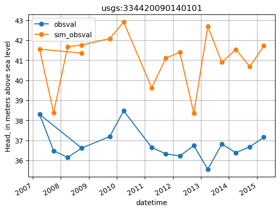
plot base data for a site
[16]:
site = 'usgs:334420090140101'
site_values = base_obs.loc[base_obs.obsprefix == site, ['datetime', 'obsval', 'sim_obsval', 'obsnme']].copy()
site_values.index = site_values.datetime
ax = site_values[['obsval', 'sim_obsval']].plot(marker='o')
ax.set_title(site)
ax.set_ylabel('Head, in meters above sea level')
ax.grid()
Changes in head through time
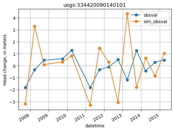
The base values returned by get_head_obs can be processed further into temporal head differences:
similar to
get_head_obstheget_temporal_differencesfunction can also write an instruction file in tandemby default, sequential differences are computed by subtracting the previous time from the current, so a positive value indicates an increase.
Sequential difference observations can help inform PEST about seasonal trends in the observation data.
[17]:
from mfobs.obs import get_temporal_differences

thead_diffs = get_temporal_differences(base_obs,
                                       perioddata,
                                       obs_values_col='obsval',
                                       sim_values_col='sim_obsval',
                                       variable='head',
                                       write_ins=True,
                                       outfile=output_folder / 'processed_head_obs_tdiffs.dat')
wrote 354 observations to output/processed_head_obs_tdiffs.dat
wrote 354 observation instructions to output/processed_head_obs_tdiffs.dat.ins
plot temporal head differences for a site
[18]:
site = 'usgs:334420090140101'
site_values = thead_diffs.loc[thead_diffs.obsprefix == site, ['datetime', 'obsval', 'sim_obsval', 'obsnme']].copy()
site_values.index = site_values.datetime
ax = site_values[['obsval', 'sim_obsval']].plot(marker='o')
ax.set_title(site)
ax.set_ylabel('Head change, in meters')
ax.grid()
Displacement in head through time
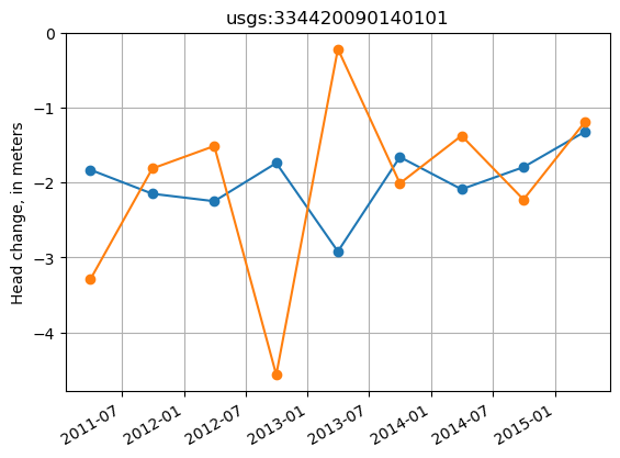
The get_temporal_differences function can also be used to compute displacement (total change) from a reference time, via the get_displacement flag.
Displacements are computed at sites with 2 or more observations.
The reference time is specified by the
displacement_fromargument.The first observation at each site that occurs on or after the reference time is then used as the datum in computing the displacements.
If no reference time is specified, the first observation is used as the datum for each site.
Displacement observations can help inform PEST about longer-term temporal trends in the observation data.
[19]:
base_obs
[19]:
| datetime | per | site_no | obsprefix | obsnme | obsval | sim_obsval | n | screen_top | screen_botm | min_layer | max_layer | i | j | obgnme | |
|---|---|---|---|---|---|---|---|---|---|---|---|---|---|---|---|
| obsnme | |||||||||||||||
| usgs:333145090261901_201409 | 2014-09-30 | 16 | USGS:333145090261901 | usgs:333145090261901 | usgs:333145090261901_201409 | 20.906667 | 28.948243 | 27 | -28.20 | -28.20 | 5 | 5 | -28 | 11 | head |
| usgs:333145090261901_201503 | 2015-03-31 | 17 | USGS:333145090261901 | usgs:333145090261901 | usgs:333145090261901_201503 | 20.985000 | 29.139873 | 181 | -28.20 | -28.20 | 5 | 5 | -28 | 11 | head |
| usgs:333145090261901_201509 | 2015-09-30 | 18 | USGS:333145090261901 | usgs:333145090261901 | usgs:333145090261901_201509 | 21.060000 | 29.057986 | 181 | -28.20 | -28.20 | 5 | 5 | -28 | 11 | head |
| usgs:333218090271101_ss | 2008-09-30 | 0 | USGS:333218090271101 | usgs:333218090271101 | usgs:333218090271101_ss | 19.320000 | 30.279858 | 2 | -102.15 | -114.34 | 6 | 6 | -27 | 10 | head |
| usgs:333218090271101_200703 | 2007-03-31 | 1 | USGS:333218090271101 | usgs:333218090271101 | usgs:333218090271101_200703 | 20.111250 | 28.161395 | 8 | -102.15 | -114.34 | 6 | 6 | -27 | 10 | head |
| ... | ... | ... | ... | ... | ... | ... | ... | ... | ... | ... | ... | ... | ... | ... | ... |
| usgs:334420090291001_201003 | 2010-03-31 | 7 | USGS:334420090291001 | usgs:334420090291001 | usgs:334420090291001_201003 | 24.135000 | 32.034462 | 2 | -58.18 | -70.38 | 5 | 5 | -5 | 6 | head |
| usgs:334420090291001_201103 | 2011-03-31 | 9 | USGS:334420090291001 | usgs:334420090291001 | usgs:334420090291001_201103 | 23.420000 | 31.645829 | 1 | -58.18 | -70.38 | 5 | 5 | -5 | 6 | head |
| usgs:334420090291001_201109 | 2011-09-30 | 10 | USGS:334420090291001 | usgs:334420090291001 | usgs:334420090291001_201109 | 23.980000 | 30.984178 | 1 | -58.18 | -70.38 | 5 | 5 | -5 | 6 | head |
| usgs:334420090291001_201203 | 2012-03-31 | 11 | USGS:334420090291001 | usgs:334420090291001 | usgs:334420090291001_201203 | 23.300000 | 31.398889 | 1 | -58.18 | -70.38 | 5 | 5 | -5 | 6 | head |
| usgs:334420090291001_201209 | 2012-09-30 | 12 | USGS:334420090291001 | usgs:334420090291001 | usgs:334420090291001_201209 | 23.780000 | 30.833197 | 1 | -58.18 | -70.38 | 5 | 5 | -5 | 6 | head |
414 rows × 15 columns
[20]:
thead_disp = get_temporal_differences(base_obs,
                                       perioddata,
                                       obs_values_col='obsval',
                                       sim_values_col='sim_obsval',
                                       variable='head',
                                       get_displacements=True,
                                       displacement_from='2010-01-01',
                                       write_ins=True,
                                       outfile=output_folder / 'processed_head_obs_disp.dat')
wrote 202 observations to output/processed_head_obs_disp.dat
wrote 202 observation instructions to output/processed_head_obs_disp.dat.ins
Plot the displacement observations
Note: the datum observation (where displacement is zero) is excluded.
[21]:
site = 'usgs:334420090140101'
site_values = thead_disp.loc[thead_disp.obsprefix == site, ['datetime', 'obsval', 'sim_obsval', 'obsnme']].copy()

# for some reason, pd.DataFrame.plot() incorrectly shifts the xticks in this case
fig, ax = plt.subplots()
ax.plot(site_values.datetime, site_values.obsval, marker='o')
ax.plot(site_values.datetime, site_values.sim_obsval, marker='o')
ax.set_title(site)
ax.set_ylabel('Head change, in meters')
fig.autofmt_xdate()
ax.grid()
Head differences between sites
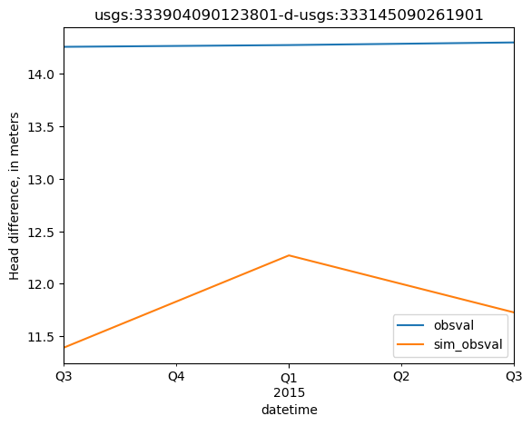
Similarly, the base values returned by get_head_obs can also be processed into spatial head differences. These may represent nested wells, well-lake differences or simply two nearby wells that represent an important head gradient.
similar to
get_head_obstheget_spatial_differencesfunction can also write an instruction file in tandem
[22]:
from mfobs.obs import get_spatial_differences

head_difference_sites = {'usgs:333904090123801':  # well in money, ms
                         'usgs:333145090261901'  # well approx. 15 mi southwest in cone of depression
                             }

shead_diffs = get_spatial_differences(base_obs,
                                      perioddata,
                                      difference_sites=head_difference_sites,
                                      obs_values_col='obsval',
                                      sim_values_col='sim_obsval',
                                      write_ins=True,
                                      outfile=output_folder / 'processed_head_obs_sdiffs.dat')
wrote 3 observations to output/processed_head_obs_sdiffs.dat
wrote 3 observation instructions to output/processed_head_obs_sdiffs.dat.ins
[23]:
shead_diffs.head()
[23]:
| datetime | per | obsprefix | obsnme1 | base_obsval1 | base_sim_obsval1 | screen_top1 | screen_botm1 | obsnme2 | base_obsval2 | base_sim_obsval2 | screen_top2 | screen_botm2 | obs_diff | sim_diff | obsnme | obsval | sim_obsval | obgnme | type | |
|---|---|---|---|---|---|---|---|---|---|---|---|---|---|---|---|---|---|---|---|---|
| per | ||||||||||||||||||||
| 16 | 2014-09-30 | 16 | usgs:333904090123801-d-usgs:333145090261901 | usgs:333904090123801_201409 | 35.163333 | 40.340913 | 23.15 | 10.96 | usgs:333145090261901_201409 | 20.906667 | 28.948243 | -28.2 | -28.2 | 14.256667 | 11.392670 | usgs:333904090123801-d-usgs:333145090261901_20... | 14.256667 | 11.392670 | head_sdiff | spatial difference |
| 17 | 2015-03-31 | 17 | usgs:333904090123801-d-usgs:333145090261901 | usgs:333904090123801_201503 | 35.258333 | 41.410755 | 23.15 | 10.96 | usgs:333145090261901_201503 | 20.985000 | 29.139873 | -28.2 | -28.2 | 14.273333 | 12.270882 | usgs:333904090123801-d-usgs:333145090261901_20... | 14.273333 | 12.270882 | head_sdiff | spatial difference |
| 18 | 2015-09-30 | 18 | usgs:333904090123801-d-usgs:333145090261901 | usgs:333904090123801_201509 | 35.358333 | 40.785719 | 23.15 | 10.96 | usgs:333145090261901_201509 | 21.060000 | 29.057986 | -28.2 | -28.2 | 14.298333 | 11.727733 | usgs:333904090123801-d-usgs:333145090261901_20... | 14.298333 | 11.727733 | head_sdiff | spatial difference |
[24]:
site = shead_diffs.obsprefix.values[0]
site_values = shead_diffs.loc[shead_diffs.obsprefix == site, ['datetime', 'obsval', 'sim_obsval', 'obsnme']].copy()
site_values.index = site_values.datetime
ax = site_values[['obsval', 'sim_obsval']].plot()
ax.set_title(site)
ax.set_ylabel('Head difference, in meters')
[24]:
Text(0, 0.5, 'Head difference, in meters')
Create a base set of flux observations
similar to head observations, the first step in flux observation processing is to create a set of base observations
observation data and model output are read and matched
by location using the
obsprefixnamesin time by averaging observed values to the model stress period
optionally, a model stress period can be labeled as steady-state (
label_period_as_steady_state), representing average conditions over a time period bracked by asteady_state_period_startandsteady_state_period_end. In this case, the simulated values for the labeled stress period are matched to average values for the steady-state time period.
observation names to match observed values to their simulated equivalents are constructed in the format of
<obsprefix>_<date suffix>, where obsprefix is a site identifier taken from theobserved_values_site_id_colinobserved_values_file, and the date suffix is controlled by theobsnme_date_suffix_formatparameter (default of'%Y%m'). Steady-state observations are assigned a suffix of'ss'.simulated and observed values are written to columns formatted with
sim_orobs_<variable_name>
[25]:
fluxobs_output_file
[25]:
PosixPath('../mfobs/tests/data/shellmound/shellmound.sfr.obs.output.csv')
[26]:
from mfobs.obs import get_base_obs
from mfobs.modflow import get_mf6_single_variable_obs

# first read the MF6 SFR package results into a dataframe
# with the appropriate formatting for get_base_obs
sfr_results = get_mf6_single_variable_obs(perioddata,
                                          model_output_file=fluxobs_output_file,
                                          )

base_flux_obs = get_base_obs(perioddata,
                             model_output=sfr_results,
                             observed_values_file=flux_obs,
                             observed_values_site_id_col='site_no',
                             observed_values_datetime_col='datetime',
                             observed_values_obsval_col='obsval',
                             label_period_as_steady_state=0,
                             steady_state_period_start=steady_state_period_start,
                             steady_state_period_end=steady_state_period_end,
                             write_ins=True,
                             outfile=output_folder / 'processed_flux_obs.dat'
                             )
base_flux_obs.head()
reading model output from ../mfobs/tests/data/shellmound/shellmound.sfr.obs.output.csv...
took 0.00s

Dropping 1 sites with no information
wrote 53 observations to output/processed_flux_obs.dat
wrote 53 observation instructions to output/processed_flux_obs.dat.ins
/home/runner/work/modflow-obs/modflow-obs/mfobs/obs.py:529: FutureWarning: Downcasting object dtype arrays on .fillna, .ffill, .bfill is deprecated and will change in a future version. Call result.infer_objects(copy=False) instead. To opt-in to the future behavior, set `pd.set_option('future.no_silent_downcasting', True)`
  base_obs.fillna(-1e30).to_csv(outfile, sep=' ', index=False)
[26]:
| datetime | per | site_no | obsprefix | obsnme | obsval | sim_obsval | obgnme | |
|---|---|---|---|---|---|---|---|---|
| obsnme | ||||||||
| 07281600_ss | 2008-09-30 | 0 | 07281600 | 07281600 | 07281600_ss | 1.349688e+07 | 6290400.0 | None |
| 07281600_200803 | 2008-03-31 | 3 | 07281600 | 07281600 | 07281600_200803 | 8.919390e+06 | 7155800.0 | None |
| 07281600_200809 | 2008-09-30 | 4 | 07281600 | 07281600 | 07281600_200809 | 1.349688e+07 | 6290400.0 | None |
| 07281600_200903 | 2009-03-31 | 5 | 07281600 | 07281600 | 07281600_200903 | 1.547445e+07 | 6740000.0 | None |
| 07281600_200909 | 2009-09-30 | 6 | 07281600 | 07281600 | 07281600_200909 | 1.365627e+07 | 7182900.0 | None |
[27]:
base_flux_obs.obsprefix.unique()
[27]:
array(['07281600', '07288280', '07288500'], dtype=object)
[28]:
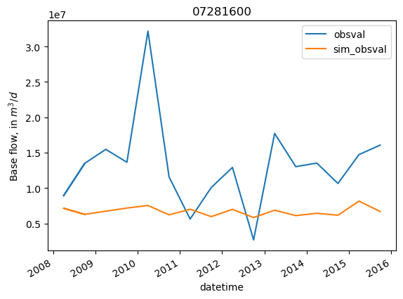
site = '07281600'
site_values = base_flux_obs.loc[base_flux_obs.obsprefix == site, ['datetime', 'obsval', 'sim_obsval', 'obsnme']].copy()
site_values.index = site_values.datetime
ax = site_values[['obsval', 'sim_obsval']].plot()
ax.set_title(site)
ax.set_ylabel('Base flow, in $m^3/d$')
[28]:
Text(0, 0.5, 'Base flow, in $m^3/d$')
Changes in streamflow through time
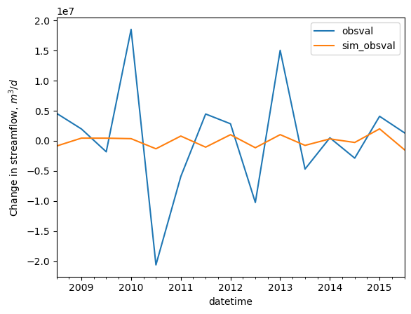
Similar to heads, the get_temporal_differences function can be used to create observations of the changes in streamflow through time at each site.
Differences are computed by subtracting the previous time from the current, so a positive value indicates an increase.
[29]:
base_flux_obs
[29]:
| datetime | per | site_no | obsprefix | obsnme | obsval | sim_obsval | obgnme | |
|---|---|---|---|---|---|---|---|---|
| obsnme | ||||||||
| 07281600_ss | 2008-09-30 | 0 | 07281600 | 07281600 | 07281600_ss | 1.349688e+07 | 6290400.0 | None |
| 07281600_200803 | 2008-03-31 | 3 | 07281600 | 07281600 | 07281600_200803 | 8.919390e+06 | 7155800.0 | None |
| 07281600_200809 | 2008-09-30 | 4 | 07281600 | 07281600 | 07281600_200809 | 1.349688e+07 | 6290400.0 | None |
| 07281600_200903 | 2009-03-31 | 5 | 07281600 | 07281600 | 07281600_200903 | 1.547445e+07 | 6740000.0 | None |
| 07281600_200909 | 2009-09-30 | 6 | 07281600 | 07281600 | 07281600_200909 | 1.365627e+07 | 7182900.0 | None |
| 07281600_201003 | 2010-03-31 | 7 | 07281600 | 07281600 | 07281600_201003 | 3.217932e+07 | 7544900.0 | None |
| 07281600_201009 | 2010-09-30 | 8 | 07281600 | 07281600 | 07281600_201009 | 1.156270e+07 | 6223100.0 | None |
| 07281600_201103 | 2011-03-31 | 9 | 07281600 | 07281600 | 07281600_201103 | 5.627040e+06 | 7018200.0 | None |
| 07281600_201109 | 2011-09-30 | 10 | 07281600 | 07281600 | 07281600_201109 | 1.008706e+07 | 5969700.0 | None |
| 07281600_201203 | 2012-03-31 | 11 | 07281600 | 07281600 | 07281600_201203 | 1.292090e+07 | 6991600.0 | None |
| 07281600_201209 | 2012-09-30 | 12 | 07281600 | 07281600 | 07281600_201209 | 2.679248e+06 | 5844400.0 | None |
| 07281600_201303 | 2013-03-31 | 13 | 07281600 | 07281600 | 07281600_201303 | 1.772296e+07 | 6874300.0 | None |
| 07281600_201309 | 2013-09-30 | 14 | 07281600 | 07281600 | 07281600_201309 | 1.303247e+07 | 6117900.0 | None |
| 07281600_201403 | 2014-03-31 | 15 | 07281600 | 07281600 | 07281600_201403 | 1.353548e+07 | 6442100.0 | None |
| 07281600_201409 | 2014-09-30 | 16 | 07281600 | 07281600 | 07281600_201409 | 1.065890e+07 | 6171300.0 | None |
| 07281600_201503 | 2015-03-31 | 17 | 07281600 | 07281600 | 07281600_201503 | 1.473788e+07 | 8164100.0 | None |
| 07281600_201509 | 2015-09-30 | 18 | 07281600 | 07281600 | 07281600_201509 | 1.607698e+07 | 6688300.0 | None |
| 07288280_ss | 2008-09-30 | 0 | 07288280 | 07288280 | 07288280_ss | 2.745655e+05 | 0.0 | None |
| 07288280_200703 | 2007-03-31 | 1 | 07288280 | 07288280 | 07288280_200703 | 1.069265e+06 | 0.0 | None |
| 07288280_200709 | 2007-09-30 | 2 | 07288280 | 07288280 | 07288280_200709 | 3.478525e+05 | 0.0 | None |
| 07288280_200803 | 2008-03-31 | 3 | 07288280 | 07288280 | 07288280_200803 | 2.555816e+05 | 0.0 | None |
| 07288280_200809 | 2008-09-30 | 4 | 07288280 | 07288280 | 07288280_200809 | 2.745655e+05 | 0.0 | None |
| 07288280_200903 | 2009-03-31 | 5 | 07288280 | 07288280 | 07288280_200903 | 2.805353e+05 | 0.0 | None |
| 07288280_200909 | 2009-09-30 | 6 | 07288280 | 07288280 | 07288280_200909 | 5.704373e+05 | 0.0 | None |
| 07288280_201003 | 2010-03-31 | 7 | 07288280 | 07288280 | 07288280_201003 | 1.596739e+06 | 0.0 | None |
| 07288280_201009 | 2010-09-30 | 8 | 07288280 | 07288280 | 07288280_201009 | 2.497488e+05 | 0.0 | None |
| 07288280_201103 | 2011-03-31 | 9 | 07288280 | 07288280 | 07288280_201103 | 1.064802e+05 | 0.0 | None |
| 07288280_201109 | 2011-09-30 | 10 | 07288280 | 07288280 | 07288280_201109 | 2.067107e+05 | 0.0 | None |
| 07288280_201203 | 2012-03-31 | 11 | 07288280 | 07288280 | 07288280_201203 | 3.397002e+05 | 0.0 | None |
| 07288280_201209 | 2012-09-30 | 12 | 07288280 | 07288280 | 07288280_201209 | 1.080637e+05 | 0.0 | None |
| 07288280_201303 | 2013-03-31 | 13 | 07288280 | 07288280 | 07288280_201303 | 2.233306e+05 | 0.0 | None |
| 07288280_201309 | 2013-09-30 | 14 | 07288280 | 07288280 | 07288280_201309 | 3.354905e+05 | 0.0 | None |
| 07288280_201403 | 2014-03-31 | 15 | 07288280 | 07288280 | 07288280_201403 | 2.422443e+05 | 0.0 | None |
| 07288280_201409 | 2014-09-30 | 16 | 07288280 | 07288280 | 07288280_201409 | 2.579483e+05 | 0.0 | None |
| 07288280_201503 | 2015-03-31 | 17 | 07288280 | 07288280 | 07288280_201503 | 9.891381e+05 | 0.0 | None |
| 07288280_201509 | 2015-09-30 | 18 | 07288280 | 07288280 | 07288280_201509 | 4.557125e+05 | 0.0 | None |
| 07288500_ss | 2008-09-30 | 0 | 07288500 | 07288500 | 07288500_ss | 8.167170e+05 | 0.0 | None |
| 07288500_200803 | 2008-03-31 | 3 | 07288500 | 07288500 | 07288500_200803 | 4.251600e+05 | 0.0 | None |
| 07288500_200809 | 2008-09-30 | 4 | 07288500 | 07288500 | 07288500_200809 | 8.167170e+05 | 0.0 | None |
| 07288500_200903 | 2009-03-31 | 5 | 07288500 | 07288500 | 07288500_200903 | 4.680965e+05 | 0.0 | None |
| 07288500_200909 | 2009-09-30 | 6 | 07288500 | 07288500 | 07288500_200909 | 9.767105e+05 | 0.0 | None |
| 07288500_201003 | 2010-03-31 | 7 | 07288500 | 07288500 | 07288500_201003 | 2.503657e+06 | 0.0 | None |
| 07288500_201009 | 2010-09-30 | 8 | 07288500 | 07288500 | 07288500_201009 | 4.230712e+05 | 0.0 | None |
| 07288500_201103 | 2011-03-31 | 9 | 07288500 | 07288500 | 07288500_201103 | 1.219689e+05 | 0.0 | None |
| 07288500_201109 | 2011-09-30 | 10 | 07288500 | 07288500 | 07288500_201109 | 3.340273e+05 | 0.0 | None |
| 07288500_201203 | 2012-03-31 | 11 | 07288500 | 07288500 | 07288500_201203 | 5.342074e+05 | 0.0 | None |
| 07288500_201209 | 2012-09-30 | 12 | 07288500 | 07288500 | 07288500_201209 | 2.296468e+05 | 0.0 | None |
| 07288500_201303 | 2013-03-31 | 13 | 07288500 | 07288500 | 07288500_201303 | 5.800736e+05 | 0.0 | None |
| 07288500_201309 | 2013-09-30 | 14 | 07288500 | 07288500 | 07288500_201309 | 8.871058e+05 | 0.0 | None |
| 07288500_201403 | 2014-03-31 | 15 | 07288500 | 07288500 | 07288500_201403 | 6.518142e+05 | 0.0 | None |
| 07288500_201409 | 2014-09-30 | 16 | 07288500 | 07288500 | 07288500_201409 | 8.534180e+05 | 0.0 | None |
| 07288500_201503 | 2015-03-31 | 17 | 07288500 | 07288500 | 07288500_201503 | 8.822385e+05 | 0.0 | None |
| 07288500_201509 | 2015-09-30 | 18 | 07288500 | 07288500 | 07288500_201509 | 6.059555e+05 | 0.0 | None |
[30]:
flux_tdiff = get_temporal_differences(base_flux_obs,
                                      perioddata,
                                      obs_values_col='obsval',
                                      sim_values_col='sim_obsval',
                                      variable='flux',
                                      write_ins=True,
                                      outfile=output_folder / 'processed_flux_obs_tdiffs.dat')
wrote 47 observations to output/processed_flux_obs_tdiffs.dat
wrote 47 observation instructions to output/processed_flux_obs_tdiffs.dat.ins
[31]:
flux_tdiff.head()
[31]:
| datetime | per | obsprefix | obsnme | obs_flux | sim_flux | obsval | sim_obsval | obgnme | type | |
|---|---|---|---|---|---|---|---|---|---|---|
| 1 | 2008-09-30 | 4 | 07281600 | 07281600_200809d200803 | 1.349688e+07 | 6290400.0 | 4.577493e+06 | -865400.0 | None_tdiff | temporal flux difference |
| 2 | 2009-03-31 | 5 | 07281600 | 07281600_200903d200809 | 1.547445e+07 | 6740000.0 | 1.977567e+06 | 449600.0 | None_tdiff | temporal flux difference |
| 3 | 2009-09-30 | 6 | 07281600 | 07281600_200909d200903 | 1.365627e+07 | 7182900.0 | -1.818178e+06 | 442900.0 | None_tdiff | temporal flux difference |
| 4 | 2010-03-31 | 7 | 07281600 | 07281600_201003d200909 | 3.217932e+07 | 7544900.0 | 1.852304e+07 | 362000.0 | None_tdiff | temporal flux difference |
| 5 | 2010-09-30 | 8 | 07281600 | 07281600_201009d201003 | 1.156270e+07 | 6223100.0 | -2.061661e+07 | -1321800.0 | None_tdiff | temporal flux difference |
[32]:
flux_tdiff.index = flux_tdiff.datetime
site = '07281600'
site_data = flux_tdiff.loc[flux_tdiff.obsprefix == site].copy()
ax = site_data[['obsval', 'sim_obsval']].plot()
ax.set_ylabel('Change in streamflow, $m^3/d$')
[32]:
Text(0, 0.5, 'Change in streamflow, $m^3/d$')
Change in streamflow between two sites
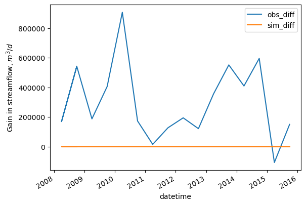
Similar to heads, the get_spatial_differences function can be used to difference stream flows between sites to create observations of stream flow gain or loss.
Differences are computed by subtracting the values site(s) from the key site, so for example, to represent a gain in streamflow as positive, the downstream site should be key site.
[33]:
flux_difference_sites = {'07288500':   # sunflower r. at sunflower
                         '07288280'  # sunflower r. at merigold
                         }

flux_sdiff = get_spatial_differences(base_flux_obs, perioddata,
                                     flux_difference_sites,
                                     obs_values_col='obsval',
                                     sim_values_col='sim_obsval',
                                     write_ins=True,
                                     outfile=output_folder / 'processed_flux_obs_sdiffs.dat')
wrote 17 observations to output/processed_flux_obs_sdiffs.dat
wrote 17 observation instructions to output/processed_flux_obs_sdiffs.dat.ins
[34]:
flux_sdiff.head()
[34]:
| datetime | per | obsprefix | obsnme1 | base_obsval1 | base_sim_obsval1 | obsnme2 | base_obsval2 | base_sim_obsval2 | obs_diff | sim_diff | obsnme | obsval | sim_obsval | obgnme | type | |
|---|---|---|---|---|---|---|---|---|---|---|---|---|---|---|---|---|
| per | ||||||||||||||||
| 0 | 2008-09-30 | 0 | 07288500-d-07288280 | 07288500_ss | 816717.0 | 0.0 | 07288280_ss | 274565.500000 | 0.0 | 542151.500000 | 0.0 | 07288500-d-07288280_ss | 542151.500000 | 0.0 | None_sdiff | spatial difference |
| 3 | 2008-03-31 | 3 | 07288500-d-07288280 | 07288500_200803 | 425160.0 | 0.0 | 07288280_200803 | 255581.650000 | 0.0 | 169578.350000 | 0.0 | 07288500-d-07288280_200803 | 169578.350000 | 0.0 | None_sdiff | spatial difference |
| 4 | 2008-09-30 | 4 | 07288500-d-07288280 | 07288500_200809 | 816717.0 | 0.0 | 07288280_200809 | 274565.500000 | 0.0 | 542151.500000 | 0.0 | 07288500-d-07288280_200809 | 542151.500000 | 0.0 | None_sdiff | spatial difference |
| 5 | 2009-03-31 | 5 | 07288500-d-07288280 | 07288500_200903 | 468096.5 | 0.0 | 07288280_200903 | 280535.333333 | 0.0 | 187561.166667 | 0.0 | 07288500-d-07288280_200903 | 187561.166667 | 0.0 | None_sdiff | spatial difference |
| 6 | 2009-09-30 | 6 | 07288500-d-07288280 | 07288500_200909 | 976710.5 | 0.0 | 07288280_200909 | 570437.333333 | 0.0 | 406273.166667 | 0.0 | 07288500-d-07288280_200909 | 406273.166667 | 0.0 | None_sdiff | spatial difference |
[35]:
flux_sdiff.index = flux_sdiff.datetime
ax = flux_sdiff[['obs_diff', 'sim_diff']].plot()
ax.set_ylabel('Gain in streamflow, $m^3/d$')
[35]:
Text(0, 0.5, 'Gain in streamflow, $m^3/d$')
[ ]: