Plotting MODFLOW listing file budgets
This notebook shows how to
make stacked bar chart summaries of MODFLOW water budgets by stress period, including global budgets and budgets for advanced stress packages (SFR, Lake, etc).
make stacked bar charts of net fluxes for each variable
plot time series of individual terms (e.g. model packages, or advanced stress package variables)
[1]:
from pathlib import Path
from mfexport.listfile import plot_list_budget, get_listfile_data, plot_budget_summary, plot_budget_term
import matplotlib.pyplot as plt
%matplotlib inline
Example MODFLOW-NWT model with monthly stress periods
[2]:
listfile = Path('data/lpr/lpr_inset.list')
model_name = listfile.stem
model_start_date='2010-12-31'

output_path = 'output'
Example MODFLOW 6 model with biannual stress periods
[3]:
mf6_listfile = Path('../mfexport/tests/data/shellmound/shellmound.list')
mf6_model_name = listfile.stem
mf6_model_start_date='1998-04-01'

output_path = 'output'
Parse the listing file budget to a dataframe
no
budgetkeyargument returns the global mass balancealternatively, use an identifying
budgetkey(text string from the listing file) to get the terms for an advanced stress package
[4]:
df = get_listfile_data(listfile=listfile, model_start_datetime=model_start_date)
df.head()
[4]:
| STORAGE_IN | CONSTANT_HEAD_IN | WELLS_IN | RECHARGE_IN | STREAM_LEAKAGE_IN | TOTAL_IN | STORAGE_OUT | CONSTANT_HEAD_OUT | WELLS_OUT | RECHARGE_OUT | STREAM_LEAKAGE_OUT | TOTAL_OUT | IN-OUT | PERCENT_DISCREPANCY | kstp | kper | |
|---|---|---|---|---|---|---|---|---|---|---|---|---|---|---|---|---|
| 2011-01-31 | 426492.593750 | 6.469874e+05 | 0.0 | 4.471989e+02 | 555.530518 | 1074482.750 | 0.000000e+00 | 394497.15625 | 81550.476562 | 0.0 | 598601.3750 | 1074649.000 | -166.250 | -0.02 | 4 | 0 |
| 2011-02-28 | 483469.062500 | 6.166172e+05 | 0.0 | 4.410000e+02 | 1439.527466 | 1101966.750 | 0.000000e+00 | 502048.40625 | 71357.640625 | 0.0 | 528673.3125 | 1102079.375 | -112.625 | -0.01 | 4 | 1 |
| 2011-03-31 | 198845.421875 | 6.208312e+05 | 0.0 | 2.617255e+05 | 1598.823853 | 1083001.125 | 1.075373e+03 | 494819.87500 | 73988.679688 | 0.0 | 513919.3125 | 1083803.250 | -802.125 | -0.07 | 4 | 2 |
| 2011-04-30 | 13266.375977 | 6.350020e+05 | 0.0 | 7.910498e+05 | 669.892212 | 1439988.000 | 4.185641e+05 | 384565.34375 | 69679.789062 | 0.0 | 567054.6250 | 1439863.750 | 124.250 | 0.01 | 4 | 3 |
| 2011-05-31 | 0.000000 | 1.154976e+06 | 0.0 | 2.851267e+06 | 0.000000 | 4006243.000 | 2.526834e+06 | 307455.37500 | 303679.531250 | 0.0 | 868731.3750 | 4006700.500 | -457.500 | -0.01 | 4 | 4 |
[5]:
mf6_df = get_listfile_data(listfile=mf6_listfile, model_start_datetime=mf6_model_start_date,
                           )
mf6_df.head()
[5]:
| STO-SS_IN | STO-SY_IN | WEL_IN | RCH_IN | SFR_IN | TOTAL_IN | STO-SS_OUT | STO-SY_OUT | WEL_OUT | RCH_OUT | SFR_OUT | TOTAL_OUT | IN-OUT | PERCENT_DISCREPANCY | kstp | kper | |
|---|---|---|---|---|---|---|---|---|---|---|---|---|---|---|---|---|
| 1998-04-02 | 0.000000 | 0.000000 | 0.0 | 358429.78125 | 1.019368e+06 | 1377797.250 | 0.000000 | 0.000000 | 0.000000 | 0.0 | 1.378546e+06 | 1378546.000 | -748.76062 | -0.05 | 0 | 0 |
| 2007-04-02 | 6.829200 | 2415.879150 | 0.0 | 358429.78125 | 1.288051e+06 | 1648903.875 | 0.000000 | 0.000000 | 500968.875000 | 0.0 | 1.147937e+06 | 1648906.125 | -2.27980 | -0.00 | 9 | 1 |
| 2007-10-02 | 1141.329956 | 381346.062500 | 0.0 | 253336.90625 | 7.053851e+05 | 1341209.375 | 27.621799 | 10508.920898 | 527275.625000 | 0.0 | 8.033984e+05 | 1341210.625 | -1.22870 | -0.00 | 4 | 2 |
| 2008-04-02 | 0.000000 | 0.000000 | 0.0 | 456429.18750 | 1.081024e+06 | 1537452.750 | 1518.002197 | 350718.281250 | 17584.275391 | 0.0 | 1.167628e+06 | 1537448.625 | 4.16440 | 0.00 | 4 | 3 |
| 2008-10-02 | 401.908112 | 112861.390625 | 0.0 | 320935.68750 | 1.216493e+06 | 1650692.375 | 44.325199 | 15359.580078 | 652556.437500 | 0.0 | 9.827312e+05 | 1650691.500 | 0.80590 | 0.00 | 4 | 4 |
Get an advanced stress package budget
in this case, for the SFR package
this requires a package budget to be written to the listing file (MODFLOW 6)
[6]:
sfr_df = get_listfile_data(listfile=mf6_listfile, model_start_datetime=mf6_model_start_date,
                       budgetkey='SFR BUDGET')
sfr_df.head()
[6]:
| GWF_IN | RAINFALL_IN | EVAPORATION_IN | RUNOFF_IN | EXT-INFLOW_IN | EXT-OUTFLOW_IN | STORAGE_IN | AUXILIARY_IN | TOTAL_IN | GWF_OUT | ... | RUNOFF_OUT | EXT-INFLOW_OUT | EXT-OUTFLOW_OUT | STORAGE_OUT | AUXILIARY_OUT | TOTAL_OUT | IN-OUT | PERCENT_DISCREPANCY | kstp | kper | |
|---|---|---|---|---|---|---|---|---|---|---|---|---|---|---|---|---|---|---|---|---|---|
| 1998-04-02 | 1.378638e+06 | 0.0 | 0.0 | 390723.562500 | 52337480.0 | 0.0 | 0.0 | 0.0 | 54106840.0 | 1.019311e+06 | ... | 0.0 | 0.0 | 53087528.0 | 0.0 | 0.0 | 54106840.0 | -1.490100e-08 | -0.0 | 0 | 0 |
| 2007-04-02 | 1.147938e+06 | 0.0 | 0.0 | 213503.109375 | 56911972.0 | 0.0 | 0.0 | 0.0 | 58273412.0 | 1.288051e+06 | ... | 0.0 | 0.0 | 56985364.0 | 0.0 | 0.0 | 58273412.0 | 1.490100e-08 | 0.0 | 9 | 1 |
| 2007-10-02 | 8.033963e+05 | 0.0 | 0.0 | 238699.078125 | 19438356.0 | 0.0 | 0.0 | 0.0 | 20480450.0 | 7.053850e+05 | ... | 0.0 | 0.0 | 19775066.0 | 0.0 | 0.0 | 20480450.0 | 0.000000e+00 | 0.0 | 4 | 2 |
| 2008-04-02 | 1.167627e+06 | 0.0 | 0.0 | 227403.312500 | 52732372.0 | 0.0 | 0.0 | 0.0 | 54127404.0 | 1.081026e+06 | ... | 0.0 | 0.0 | 53046380.0 | 0.0 | 0.0 | 54127404.0 | 2.235200e-08 | 0.0 | 4 | 3 |
| 2008-10-02 | 9.827311e+05 | 0.0 | 0.0 | 386176.125000 | 51699144.0 | 0.0 | 0.0 | 0.0 | 53068052.0 | 1.216493e+06 | ... | 0.0 | 0.0 | 51851560.0 | 0.0 | 0.0 | 53068052.0 | -7.450600e-09 | -0.0 | 4 | 4 |
5 rows × 22 columns
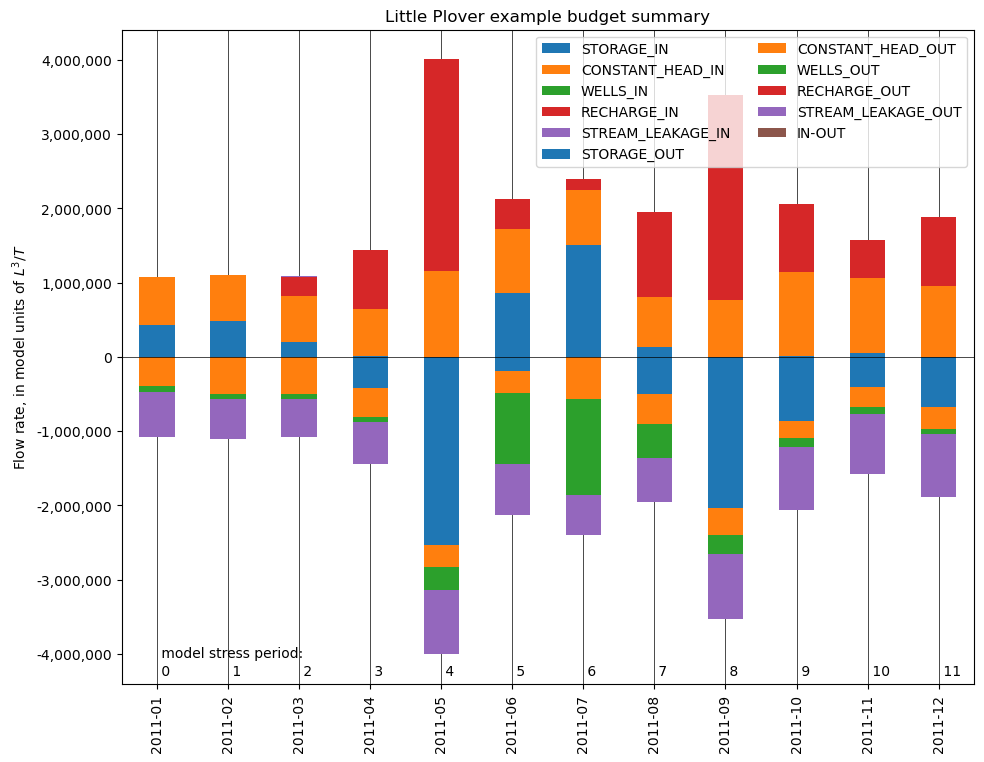
Basic summary of MODFLOW water balance
[7]:
plot_budget_summary(df, title_prefix='Little Plover example',
                    xtick_stride=1)
[7]:
<Axes: title={'center': 'Little Plover example budget summary'}, ylabel='Flow rate, in model units of $L^3/T$'>
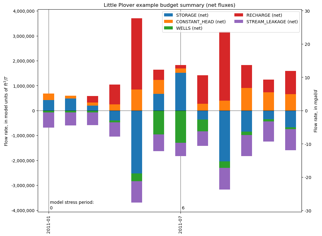
Plot just the net fluxes for each component
add a secondary axis with other units
Note: model_length_units and model_time_units are needed to convert units to the secondary axis units.
[8]:
plot_budget_summary(df, title_prefix='Little Plover example', term_nets=True,
                    model_length_units='feet', model_time_units='time',
                    secondary_axis_units='mgal/day')
[8]:
<Axes: title={'center': 'Little Plover example budget summary (net fluxes)'}, ylabel='Flow rate, in model units of $ft^3/T$'>
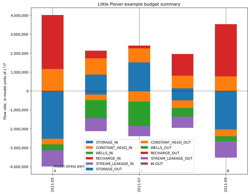
Plot a subset of results
This can be useful for models with many stress periods
[9]:
plot_budget_summary(df, title_prefix='Little Plover example',
                    xtick_stride=2,
                        plot_start_date='2011-05', plot_end_date='2011-09')
[9]:
<Axes: title={'center': 'Little Plover example budget summary'}, ylabel='Flow rate, in model units of $L^3/T$'>
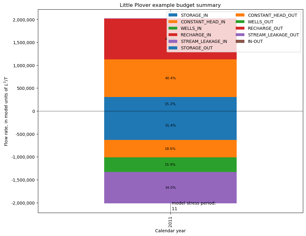
plot budget sums by calendar year
with percentages
[10]:
ax = plot_budget_summary(df, title_prefix='Little Plover example',
                         annual_sums=True, plot_pcts=True)
plot budget sums for an arbitrary grouping
plot_budget_summary and plot_budget_term can take any DataFrame with column names structured like those output by flopy.utils.MfListBudget (i.e. with _IN or _OUT suffixes), and a datetime index. So pandas groupby (or any other manipulations) can be performed on the data beforehand to achieve the desired result.
In this case, we group the data into growing season vs. non-growing season based on month:
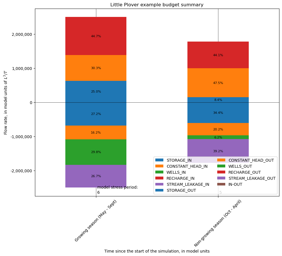
[11]:
df['growing_season'] = 'Non-growing season (Oct - April)'
df.loc[(df.index.month > 5) & (df.index.month < 10), 'growing_season'] = 'Growing season (May - Sept)'
gs = df.groupby('growing_season').mean()
gs
[11]:
| STORAGE_IN | CONSTANT_HEAD_IN | WELLS_IN | RECHARGE_IN | STREAM_LEAKAGE_IN | TOTAL_IN | STORAGE_OUT | CONSTANT_HEAD_OUT | WELLS_OUT | RECHARGE_OUT | STREAM_LEAKAGE_OUT | TOTAL_OUT | IN-OUT | PERCENT_DISCREPANCY | kstp | kper | |
|---|---|---|---|---|---|---|---|---|---|---|---|---|---|---|---|---|
| growing_season | ||||||||||||||||
| Growing season (May - Sept) | 625680.937500 | 757334.25 | 0.0 | 1.117286e+06 | 684.561279 | 2500986.00 | 681521.0000 | 406225.3750 | 746160.937500 | 0.0 | 667186.375 | 2501093.750 | -107.687500 | -0.00500 | 4.0 | 6.5 |
| Non-growing season (Oct - April) | 148805.484375 | 845780.50 | 0.0 | 7.841528e+05 | 532.971741 | 1779271.75 | 611469.8125 | 360034.9375 | 110107.578125 | 0.0 | 697856.500 | 1779468.875 | -197.078125 | -0.01375 | 4.0 | 5.0 |
[12]:
ax = plot_budget_summary(gs, title_prefix='Little Plover example',
                         plot_pcts=True)
ax.xaxis.set_tick_params(rotation=45)
This can be done for net fluxes too
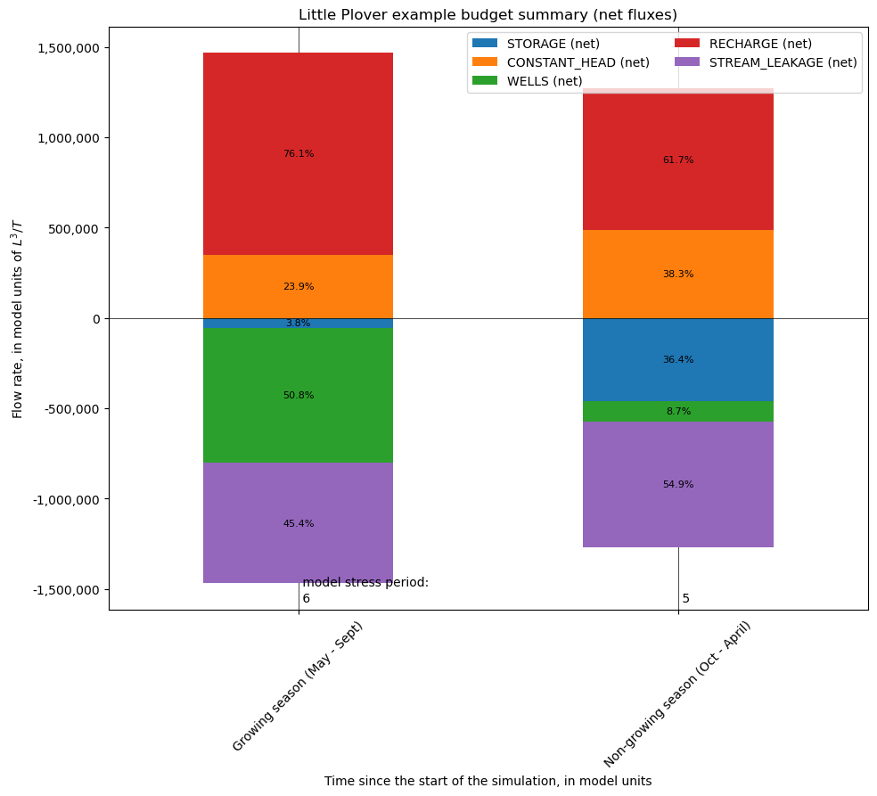
[13]:
df['growing_season'] = 'Non-growing season (Oct - April)'
df.loc[(df.index.month > 5) & (df.index.month < 10), 'growing_season'] = 'Growing season (May - Sept)'
gs = df.groupby('growing_season').mean()
ax = plot_budget_summary(gs, title_prefix='Little Plover example',
                         term_nets=True,
                         plot_pcts=True)
ax.xaxis.set_tick_params(rotation=45)
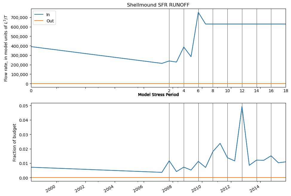
Plot a budget term
Two plots are produced * absolute values, optionally with secondary axis as above * as a fraction of model or advanced stress package (e.g. SFR) budget
[14]:
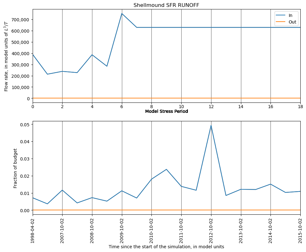
plot_budget_term(sfr_df, 'RUNOFF_IN', title_prefix='Shellmound SFR')
Any column in the listing file budget dataframe (df) can be plotted,
by specifying the first part of the column name (without the _IN or _OUT at the end)
[15]:
df.columns
[15]:
Index(['STORAGE_IN', 'CONSTANT_HEAD_IN', 'WELLS_IN', 'RECHARGE_IN',
       'STREAM_LEAKAGE_IN', 'TOTAL_IN', 'STORAGE_OUT', 'CONSTANT_HEAD_OUT',
       'WELLS_OUT', 'RECHARGE_OUT', 'STREAM_LEAKAGE_OUT', 'TOTAL_OUT',
       'IN-OUT', 'PERCENT_DISCREPANCY', 'kstp', 'kper', 'growing_season'],
      dtype='object')
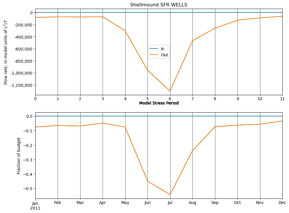
For example
[16]:
plot_budget_term(df, 'WELLS', title_prefix='Shellmound SFR')
Plot term by stress period instead of time
Can be useful for models with long spin-up periods that obscure shorter periods of interest when whole simulation time is plotted.
[17]:
plot_budget_term(sfr_df, 'RUNOFF_IN', title_prefix='Shellmound SFR',
                 plot_start_date=None, plot_end_date=None,
                 datetime_xaxis=False)
/home/runner/work/modflow-export/modflow-export/mfexport/listfile.py:670: UserWarning: set_ticklabels() should only be used with a fixed number of ticks, i.e. after set_ticks() or using a FixedLocator.
  ax2.set_xticklabels(datetime_labels, rotation=90)
Plot mass balance error
[18]:
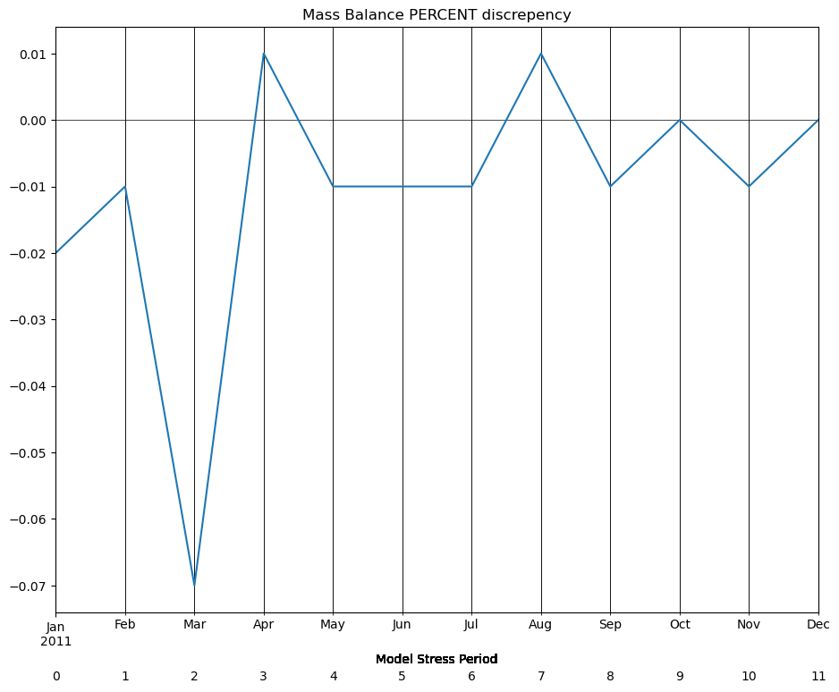
plot_budget_term(df, 'PERCENT_DISCREPANCY', title_prefix='Mass Balance',
                 title_suffix='discrepency')
Macro to plot everything to PDFs
budget summary (in/out and net)
timeseries of budget terms for each package, and within each advanced stress package
[19]:
plot_list_budget(listfile=mf6_listfile, output_path=output_path,
                 model_start_datetime='1998-04-01')
creating output/pdfs...
creating output/shps...
creating output/rasters...
wrote output/pdfs/listfile_budget_summary.pdf
wrote output/pdfs/listfile_budget_by_term.pdf
[ ]: