Note
Lake Package Example
First set the path and import the required packages. The flopy path doesn’t have to be set if you install flopy from a binary installer. If you want to run this notebook, you have to set the path to your own flopy path.
[1]:
import os
import sys
from tempfile import TemporaryDirectory

import numpy as np
import matplotlib as mpl
import matplotlib.pyplot as plt

# run installed version of flopy or add local path
try:
    import flopy
except:
    fpth = os.path.abspath(os.path.join("..", ".."))
    sys.path.append(fpth)
    import flopy

# temporary directory
temp_dir = TemporaryDirectory()
workspace = temp_dir.name

print(sys.version)
print("numpy version: {}".format(np.__version__))
print("matplotlib version: {}".format(mpl.__version__))
print("flopy version: {}".format(flopy.__version__))
3.10.10 | packaged by conda-forge | (main, Mar 24 2023, 20:08:06) [GCC 11.3.0]
numpy version: 1.24.3
matplotlib version: 3.7.1
flopy version: 3.3.7
We are creating a square model with a specified head equal to h1 along all boundaries. The head at the cell in the center in the top layer is fixed to h2. First, set the name of the model and the parameters of the model: the number of layers Nlay, the number of rows and columns N, lengths of the sides of the model L, aquifer thickness H, hydraulic conductivity k
[2]:
name = "lake_example"
h1 = 100
h2 = 90
Nlay = 10
N = 101
L = 400.0
H = 50.0
k = 1.0
Create a MODFLOW model and store it (in this case in the variable ml, but you can call it whatever you want). The modelname will be the name given to all MODFLOW files (input and output). The exe_name should be the full path to your MODFLOW executable. The version is either ‘mf2k’ for MODFLOW2000 or ‘mf2005’for MODFLOW2005.
[3]:
ml = flopy.modflow.Modflow(
    modelname=name, exe_name="mf2005", version="mf2005", model_ws=workspace
)
Define the discretization of the model. All layers are given equal thickness. The bot array is build from the Hlay values to indicate top and bottom of each layer, and delrow and delcol are computed from model size L and number of cells N. Once these are all computed, the Discretization file is built.
[4]:
bot = np.linspace(-H / Nlay, -H, Nlay)
delrow = delcol = L / (N - 1)
dis = flopy.modflow.ModflowDis(
    ml,
    nlay=Nlay,
    nrow=N,
    ncol=N,
    delr=delrow,
    delc=delcol,
    top=0.0,
    botm=bot,
    laycbd=0,
)
Next we specify the boundary conditions and starting heads with the Basic package. The ibound array will be 1 in all cells in all layers, except for along the boundary and in the cell at the center in the top layer where it is set to -1 to indicate fixed heads. The starting heads are used to define the heads in the fixed head cells (this is a steady simulation, so none of the other starting values matter). So we set the starting heads to h1 everywhere, except for the head at the
center of the model in the top layer.
[5]:
Nhalf = int((N - 1) / 2)
ibound = np.ones((Nlay, N, N), dtype=int)
ibound[:, 0, :] = -1
ibound[:, -1, :] = -1
ibound[:, :, 0] = -1
ibound[:, :, -1] = -1
ibound[0, Nhalf, Nhalf] = -1
start = h1 * np.ones((N, N))
start[Nhalf, Nhalf] = h2
bas = flopy.modflow.ModflowBas(ml, ibound=ibound, strt=start)
The aquifer properties (really only the hydraulic conductivity) are defined with the LPF package.
[6]:
lpf = flopy.modflow.ModflowLpf(ml, hk=k)
Finally, we need to specify the solver we want to use (PCG with default values), and the output control (using the default values). Then we are ready to write all MODFLOW input files and run MODFLOW.
[7]:
pcg = flopy.modflow.ModflowPcg(ml)
oc = flopy.modflow.ModflowOc(ml)
ml.write_input()
success, buff = ml.run_model(silent=True, report=True)
if success:
    for line in buff:
        print(line)
else:
    raise ValueError("Failed to run.")
                                  MODFLOW-2005
    U.S. GEOLOGICAL SURVEY MODULAR FINITE-DIFFERENCE GROUND-WATER FLOW MODEL
                             Version 1.12.00 2/3/2017

 Using NAME file: lake_example.nam
 Run start date and time (yyyy/mm/dd hh:mm:ss): 2023/05/04 16:00:46

 Solving:  Stress period:     1    Time step:     1    Ground-Water Flow Eqn.
 Run end date and time (yyyy/mm/dd hh:mm:ss): 2023/05/04 16:00:46
 Elapsed run time:  0.382 Seconds

  Normal termination of simulation
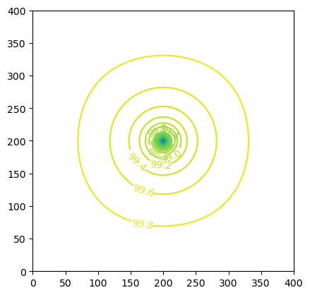
Once the model has terminated normally, we can read the heads file. First, a link to the heads file is created with HeadFile. The link can then be accessed with the get_data function, by specifying, in this case, the step number and period number for which we want to retrieve data. A three-dimensional array is returned of size nlay, nrow, ncol. Matplotlib contouring functions are used to make contours of the layers or a cross-section.
[8]:
hds = flopy.utils.HeadFile(os.path.join(workspace, name + ".hds"))
h = hds.get_data(kstpkper=(0, 0))
x = y = np.linspace(0, L, N)
c = plt.contour(x, y, h[0], np.arange(90, 100.1, 0.2))
plt.clabel(c, fmt="%2.1f")
plt.axis("scaled");
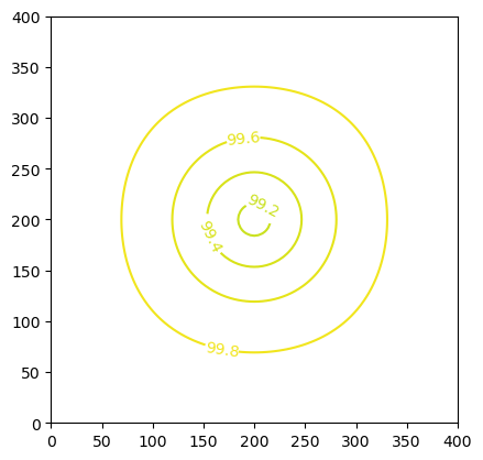
[9]:
x = y = np.linspace(0, L, N)
c = plt.contour(x, y, h[-1], np.arange(90, 100.1, 0.2))
plt.clabel(c, fmt="%1.1f")
plt.axis("scaled");
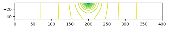
[10]:
z = np.linspace(-H / Nlay / 2, -H + H / Nlay / 2, Nlay)
c = plt.contour(x, z, h[:, 50, :], np.arange(90, 100.1, 0.2))
plt.axis("scaled");
[11]:
try:
    # ignore PermissionError on Windows
    temp_dir.cleanup()
except:
    pass