Demo of USGS-MAP-gwmodels
This page demonstrates some of the core features of USGS-MAP-gwmodel obs, applied to the Mississippi Delta inset model area. Specifically:
setup of model layering and property zones by combining voxel-based hydrogeologic facies derived from an airborne electromagnetic (AEM) survey (Burton and others, 2020) with traditional raster surfaces denoting hydrogeologic contacts (Hart and others, 2008)
culling of NetCDF-based infiltration data (Westenbroek and others, 2020) to the model area, and aggregation to monthly values
preprocessing of streamflow timeseries for use as specified inflows to the SFR package, or streamflow observations
preprocessing of head observations
preprocessing of water use data, including:
estimates of agricultural water use (Wilson, 2020)
non-agricultulral water use data from the USGS
[1]:
from pathlib import Path
import numpy as np
import pandas as pd
import xarray as xr
import matplotlib.pyplot as plt
import matplotlib as mpl
from mfsetup.grid import MFsetupGrid
Define some global inputs
[2]:
test_data_path = Path('../mapgwm/tests/data')
output_folder = Path('output')
output_folder.mkdir(exist_ok=True)  # make the output folder if it doesn't exist

# ms delta geographic extent
delta_extent = test_data_path / 'extents/ms_delta.shp'

# simulation start date
start_date='1998-04-01'

# model grid for the MS Delta inset model
ncol=270
nrow=605
dxy=500.
delr = np.ones(ncol) * dxy
delc = np.ones(nrow) * dxy
delta_inset_model_grid = MFsetupGrid(delc, delr, top=None, botm=None,
                                     lenuni=2, epsg=5070,
                                     xoff=434955, yoff=1040285, angrot=0.0)

# shapefile with polygons to group observations by geographic area
geographic_groups = [test_data_path / 'extents/CompositeHydrographArea.shp',
                     test_data_path / 'extents/MAP_generalized_regions.shp'
                     ]
Set up the model layering and property zones
from AEM-based voxel data and raster surfaces of hydrogeologic contacts
[3]:
# mean dem values for each 1 km gridcell, elevation units of feet
dem_means_raster = test_data_path / 'rasters/dem_mean_elevs_1000.tif'

# AEM electrical resistivity-based facies classes from tempest and resolve surveys
# (All facies classes version)
facies_classes_netcdf = test_data_path / 'netcdf/RSTM_res_fac_depth_15m.nc'

# Original MERAS framework (1 mi resolution), elevation units of feet
framework_rasters = [
    test_data_path / 'rasters/vkbg_surf.tif',  # Vicksburg-Jackson Group (top)
    test_data_path / 'rasters/ucaq_surf.tif',  # Upper Claiborne aquifer (top)
    test_data_path / 'rasters/mccu_surf.tif',  # Middle Claiborne confining unit (t
    test_data_path / 'rasters/mcaq_surf.tif',  # Middle Claiborne aquifer (top)
    test_data_path / 'rasters/lccu_surf.tif',  # Lower Claiborne confining unit (to
    test_data_path / 'rasters/lcaq_surf.tif',  # Lower Claiborne aquifer (top)
    test_data_path / 'rasters/mwaq_surf.tif',  # Middle Wilcox aquifer (top)
    test_data_path / 'rasters/lwaq_surf.tif',  # Lower Wilcox aquifer (top)
    test_data_path / 'rasters/mdwy_surf.tif',  # Midway confining unit (top)
]
framework_unit_names = [
    'Undifferentiated sediments\nabove the Vicksburg',
    'Vicksburg-Jackson Group',
    'Upper Claiborne aquifer',
    'Middle Claiborne confining unit',
    'Middle Claiborne aquifer',
    'Lower Claiborne confining unit',
    'Lower Claiborne aquifer',
    'Middle Wilcox aquifer',
    'Lower Wilcox aquifer'
]
[4]:
from mapgwm.framework import setup_model_layers, plot_slice

layers, zone_array = setup_model_layers(dem_means_raster,
                                        facies_classes_netcdf,
                                        framework_rasters,
                                        delta_inset_model_grid,
                                        facies_class_variable='fac_a',  # variable in facies_classes_netcdf with facies zones
                                        dem_elevation_units='feet',
                                        framework_raster_elevation_units='feet',
                                        model_length_units='meters', output_folder=output_folder,
                                        framework_unit_names=framework_unit_names)
reading data from ../mapgwm/tests/data/rasters/dem_mean_elevs_1000.tif...
finished in 0.06s
reading data from ../mapgwm/tests/data/rasters/vkbg_surf.tif...
finished in 0.03s
reading data from ../mapgwm/tests/data/rasters/ucaq_surf.tif...
finished in 0.03s
reading data from ../mapgwm/tests/data/rasters/mccu_surf.tif...
finished in 0.03s
reading data from ../mapgwm/tests/data/rasters/mcaq_surf.tif...
finished in 0.03s
reading data from ../mapgwm/tests/data/rasters/lccu_surf.tif...
finished in 0.03s
reading data from ../mapgwm/tests/data/rasters/lcaq_surf.tif...
finished in 0.03s
reading data from ../mapgwm/tests/data/rasters/mwaq_surf.tif...
finished in 0.03s
reading data from ../mapgwm/tests/data/rasters/lwaq_surf.tif...
finished in 0.02s
reading data from ../mapgwm/tests/data/rasters/mdwy_surf.tif...
finished in 0.03s
computing cell thicknesses...
finished in 6.46s

computing cell thicknesses...
finished in 14.16s

wrote output/botm_array/model_top.tif
wrote output/botm_array/botm0.tif
wrote output/botm_array/botm1.tif
wrote output/botm_array/botm2.tif
wrote output/botm_array/botm3.tif
wrote output/botm_array/botm4.tif
wrote output/botm_array/botm5.tif
wrote output/botm_array/botm6.tif
wrote output/botm_array/botm7.tif
wrote output/botm_array/botm8.tif
wrote output/botm_array/botm9.tif
wrote output/botm_array/botm10.tif
wrote output/botm_array/botm11.tif
wrote output/botm_array/botm12.tif
wrote output/botm_array/botm13.tif
wrote output/botm_array/botm14.tif
wrote output/botm_array/botm15.tif
wrote output/botm_array/botm16.tif
wrote output/botm_array/botm17.tif
wrote output/botm_array/botm18.tif
wrote output/botm_array/botm19.tif
wrote output/botm_array/botm20.tif
wrote output/botm_array/botm21.tif
wrote output/botm_array/botm22.tif
wrote output/botm_array/botm23.tif
wrote output/botm_array/botm24.tif
wrote output/botm_array/botm25.tif
wrote output/botm_array/botm26.tif
wrote output/botm_array/botm27.tif
wrote output/botm_array/botm28.tif
wrote output/botm_array/botm29.tif
wrote output/botm_array/botm30.tif
wrote output/zones/rasters/res_fac0.tif
wrote output/zones/rasters/res_fac1.tif
wrote output/zones/rasters/res_fac2.tif
wrote output/zones/rasters/res_fac3.tif
wrote output/zones/rasters/res_fac4.tif
wrote output/zones/rasters/res_fac5.tif
wrote output/zones/rasters/res_fac6.tif
wrote output/zones/rasters/res_fac7.tif
wrote output/zones/rasters/res_fac8.tif
wrote output/zones/rasters/res_fac9.tif
wrote output/zones/rasters/res_fac10.tif
wrote output/zones/rasters/res_fac11.tif
wrote output/zones/rasters/res_fac12.tif
wrote output/zones/rasters/res_fac13.tif
wrote output/zones/rasters/res_fac14.tif
wrote output/zones/rasters/res_fac15.tif
wrote output/zones/rasters/res_fac16.tif
wrote output/zones/rasters/res_fac17.tif
wrote output/zones/rasters/res_fac18.tif
wrote output/zones/rasters/res_fac19.tif
wrote output/zones/rasters/res_fac20.tif
wrote output/zones/rasters/res_fac21.tif
wrote output/zones/rasters/res_fac22.tif
wrote output/zones/rasters/res_fac23.tif
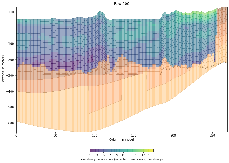
Plot a cross section slice
[5]:
framework_unit_labels = dict(zip(range(13, 32), framework_unit_names))
[6]:
plot_slice(layers, property_data=zone_array,
           row=100, column=slice(None),
           voxel_start_layer=0, voxel_zones=np.arange(1, 21), cmap='copper',
           voxel_cmap='viridis', unit_labels=framework_unit_labels)
[6]:
<AxesSubplot:title={'center':'Row 100'}, xlabel='Column in model', ylabel='Elevation, in meters'>
Preprocess recharge
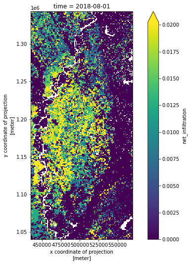
Chop the SWB source data down to the model area and aggregate daily values to monthly means
[7]:
from mapgwm.swb import get_monthly_means

data_file = test_data_path / 'swb/delta_swb_summer2018.nc'

# output
outputfile = output_folder / 'swb_monthly_means.nc'

# get the monthly means
get_monthly_means(data_file, outfile=outputfile,
                  filter=delta_inset_model_grid.bounds, check_results=True)
using dask...
opening ../mapgwm/tests/data/swb/delta_swb_summer2018.nc...
culling to bounding box: (434955.0, 1040285.0, 569955.0, 1342785.0)
Aggregating to monthly values...
wrote output/swb_monthly_means.nc
took 0.18s

checking compressed file
finished in 0.24s
[8]:
with xr.open_dataset(outputfile) as ds:
    fig, ax = plt.subplots(figsize=(11, 8.5))
    ds['net_infiltration'].sel(time='2018-08').plot(ax=ax, vmax=ds['net_infiltration'].quantile(0.95))
    ax.set_aspect(1)
Preprocess streamflow data for specified inflows to the SFR package
[9]:
from mapgwm.swflows import preprocess_flows

streamflow_data_file = test_data_path / 'swflows/13Feb2020_rf_output_with_site_numbers.csv'
streamflow_data = pd.read_csv(streamflow_data_file)

# only include flows that are inflows (exclude observations)
include_line_ids = set(streamflow_data.loc[streamflow_data.group == 'meras-inflows', 'comid'])

outfile = output_folder / 'processed_inflows.csv'
[10]:
streamflow_data.head()
[10]:
| site_no | comid | datetime | name | group | X | Y | predicted_bf | predicted_total_flow | category | |
|---|---|---|---|---|---|---|---|---|---|---|
| 0 | 07277700 | 15251676 | 2007-02-01 | HICKAHALA CREEK NR SENATOBIA, MS | meras-observations | -89.7839 | 34.6394 | 82.1099 | 107.1910 | estimated |
| 1 | 07277700 | 15251676 | 2007-03-01 | HICKAHALA CREEK NR SENATOBIA, MS | meras-observations | -89.7839 | 34.6394 | 75.3402 | 85.2905 | estimated |
| 2 | 07277700 | 15251676 | 2007-04-01 | HICKAHALA CREEK NR SENATOBIA, MS | meras-observations | -89.7839 | 34.6394 | 46.6768 | 80.6870 | estimated |
| 3 | 07277700 | 15251676 | 2007-05-01 | HICKAHALA CREEK NR SENATOBIA, MS | meras-observations | -89.7839 | 34.6394 | 41.8452 | 49.2666 | estimated |
| 4 | 07277700 | 15251676 | 2007-06-01 | HICKAHALA CREEK NR SENATOBIA, MS | meras-observations | -89.7839 | 34.6394 | 37.1356 | 47.5411 | estimated |
[11]:
data, metadata = preprocess_flows(streamflow_data, flow_data_columns=['predicted_total_flow', 'predicted_bf'],
                                  include_line_ids=include_line_ids,
                                  start_date=start_date,
                                  datetime_col='datetime',
                                  site_no_col='site_no',
                                  line_id_col='comid',
                                  x_coord_col='X',
                                  y_coord_col='Y',
                                  outfile=outfile
                                  )
writing output/processed_inflows_info.shp... Done
writing output/processed_inflows_info.csv
writing output/processed_inflows.csv
[12]:
data.head()
[12]:
| site_no | line_id | datetime | predicted_total_flow | predicted_bf | category | |
|---|---|---|---|---|---|---|
| datetime | ||||||
| 2007-02-01 | none | 19274790 | 2007-02-01 | 5.175779e+06 | 4.458664e+06 | measured |
| 2007-03-01 | none | 19274790 | 2007-03-01 | 2.497954e+06 | 1.873441e+06 | measured |
| 2007-04-01 | none | 19274790 | 2007-04-01 | 3.820059e+06 | 2.017639e+06 | measured |
| 2007-05-01 | none | 19274790 | 2007-05-01 | 2.154971e+06 | 1.052037e+06 | measured |
| 2007-06-01 | none | 19274790 | 2007-06-01 | 1.437397e+06 | 5.956531e+05 | measured |
[13]:
metadata.head()
[13]:
| start_dt | site_no | end_dt | n | x | y | line_id | name | geometry | obsprefix | group | |
|---|---|---|---|---|---|---|---|---|---|---|---|
| site_no | |||||||||||
| none | 2007-02-01 | none | 2018-12-01 | 143 | 438600.380812 | 1.105540e+06 | 19274790 | Tensas River | POINT (438600.3808115814 1105539.758365622) | none | fluxes |
Preprocess streamflow data for SFR package observations
Unlike the inflows, which are referenced by NHDPlus COMID, these all have site numbers
Additionally, we want to fill gaps in measured flow data with statistical estimates
The
dataDataFrame outputs have the time series;The
metadataDataFrame outputs have site information that can be input to ``modflow-setup`` to set up the observation input for MODFLOW-6.
[14]:
# only include flows that are inflows (exclude observations)
include_sites = set(streamflow_data.loc[streamflow_data.group == 'meras-observations', 'site_no'])

outfile = output_folder / 'processed_flow_obs.csv'

# rename these columns, if present
column_renames = {'predicted_total_flow': 'qtotal_m3d',
                  'predicted_bf': 'qbase_m3d',
                  'qbase_cfs': 'qbase_m3d',
                  'q_cfs': 'qtotal_m3d',
                  'station_nm': 'name'}
preprocess the statistical estimates
[15]:
est_data, est_metadata = preprocess_flows(streamflow_data, flow_data_columns=['predicted_total_flow', 'predicted_bf'],
                                          include_sites=include_sites,
                                          start_date=start_date,
                                          active_area=delta_extent,
                                          datetime_col='datetime',
                                          site_no_col='site_no',
                                          line_id_col='comid',
                                          x_coord_col='X',
                                          y_coord_col='Y',
                                          geographic_groups=geographic_groups,
                                          geographic_groups_col='obsgroup',
                                          flow_qualifier_column='category',
                                          source_crs=4269,
                                          dest_crs=5070,
                                          source_volume_units='ft3',
                                          source_time_units='s',
                                          dest_volume_units='m3',
                                          dest_time_units='d',
                                          column_renames=column_renames,
                                          outfile=None
                                          )
reading ../mapgwm/tests/data/extents/ms_delta.shp...
--> building dataframe... (may take a while for large shapefiles)
Culling 7 sites outside of the model area defined by ['../mapgwm/tests/data/extents/ms_delta.shp'].

reading ../mapgwm/tests/data/extents/MAP_generalized_regions.shp...
--> building dataframe... (may take a while for large shapefiles)

reading ../mapgwm/tests/data/extents/CompositeHydrographArea.shp...
--> building dataframe... (may take a while for large shapefiles)
[16]:
est_data.head()
[16]:
| site_no | line_id | datetime | qtotal_m3d | qbase_m3d | category | |
|---|---|---|---|---|---|---|
| datetime | ||||||
| 2007-02-01 | 07288847 | 17929890 | 2007-02-01 | 659171.062935 | 564867.808532 | estimated |
| 2007-03-01 | 07288847 | 17929890 | 2007-03-01 | 316339.771464 | 278767.710811 | estimated |
| 2007-04-01 | 07288847 | 17929890 | 2007-04-01 | 328301.079306 | 179244.687481 | estimated |
| 2007-05-01 | 07288847 | 17929890 | 2007-05-01 | 632789.638827 | 216849.532247 | estimated |
| 2007-06-01 | 07288847 | 17929890 | 2007-06-01 | 250184.368712 | 130957.604569 | estimated |
[17]:
est_metadata.head()
[17]:
| start_dt | site_no | end_dt | n | x | y | line_id | name | geometry | obsprefix | group | geo_group | |
|---|---|---|---|---|---|---|---|---|---|---|---|---|
| site_no | ||||||||||||
| 07288000 | 2007-02-01 | 07288000 | 2018-12-01 | 143 | 496047.363537 | 1.262247e+06 | 17951955 | Big Sunflower River | POINT (496047.3635373298 1262247.29440906) | 07288000 | fluxes | delta |
| 07288280 | 2007-02-01 | 07288280 | 2018-12-01 | 143 | 489208.729363 | 1.239410e+06 | 17958105 | BIG SUNFLOWER RIVER NR MERIGOLD, MS | POINT (489208.7293628419 1239410.03140523) | 07288280 | fluxes | delta |
| 07288555 | 2007-02-01 | 07288555 | 2018-12-01 | 143 | 509254.529536 | 1.233598e+06 | 17958153 | QUIVER RIVER SOUTHEAST RULEVILLE, MS | POINT (509254.5295362755 1233597.934250077) | 07288555 | fluxes | delta |
| 07288650 | 2007-02-01 | 07288650 | 2018-12-01 | 143 | 472484.774612 | 1.196944e+06 | 17963095 | BOGUE PHALIA NR LELAND, MS | POINT (472484.7746117859 1196943.873882911) | 07288650 | fluxes | delta |
| 07288700 | 2007-02-01 | 07288700 | 2018-12-01 | 143 | 492594.661169 | 1.195806e+06 | 17970237 | Big Sunflower River | POINT (492594.6611692713 1195806.16802324) | 07288700 | fluxes | delta |
preprocess the measured values
[18]:
nwis_streamflow_data = test_data_path / 'swflows/nwis_dvs.csv'
nwis_streamflow_metadata = test_data_path / 'swflows/nwis_dv_sites.csv'

meas_data, meas_metadata = preprocess_flows(nwis_streamflow_data, nwis_streamflow_metadata,
                                            flow_data_columns=['q_cfs', 'qbase_cfs'],
                                            include_sites=include_sites,
                                            start_date=start_date,
                                            active_area=delta_extent,
                                            datetime_col='datetime',
                                            site_no_col='site_no',
                                            line_id_col='comid',
                                            x_coord_col='dec_long_va',
                                            y_coord_col='dec_lat_va',
                                            geographic_groups=geographic_groups,
                                            geographic_groups_col='obsgroup',
                                            source_crs=4269,
                                            dest_crs=5070,
                                            source_volume_units='ft3',
                                            source_time_units='s',
                                            dest_volume_units='m3',
                                            dest_time_units='d',
                                            column_renames=column_renames,
                                            outfile=None
                                            )
reading ../mapgwm/tests/data/extents/ms_delta.shp...
--> building dataframe... (may take a while for large shapefiles)
Culling 40 sites outside of the model area defined by ['../mapgwm/tests/data/extents/ms_delta.shp'].

reading ../mapgwm/tests/data/extents/MAP_generalized_regions.shp...
--> building dataframe... (may take a while for large shapefiles)

reading ../mapgwm/tests/data/extents/CompositeHydrographArea.shp...
--> building dataframe... (may take a while for large shapefiles)
[19]:
meas_data.head()
[19]:
| site_no | datetime | qtotal_m3d | qbase_m3d | category | |
|---|---|---|---|---|---|
| datetime | |||||
| 2008-01-20 | 07280400 | 2008-01-20 | 93459.185840 | 93459.185840 | measured |
| 2008-01-21 | 07280400 | 2008-01-21 | 90278.637631 | 90278.637631 | measured |
| 2008-01-22 | 07280400 | 2008-01-22 | 153155.629151 | 92176.690939 | measured |
| 2008-01-23 | 07280400 | 2008-01-23 | 214809.332899 | 94114.868086 | measured |
| 2008-01-24 | 07280400 | 2008-01-24 | 144347.957187 | 96093.658387 | measured |
[20]:
meas_metadata.head()
[20]:
| site_no | name | site_tp_cd | y | x | coord_meth_cd | coord_acy_cd | coord_datum_cd | dec_coord_datum_cd | district_cd | ... | sv_begin_date | sv_end_date | sv_count_nu | geometry | start_dt | end_dt | n | obsprefix | group | geo_group | |
|---|---|---|---|---|---|---|---|---|---|---|---|---|---|---|---|---|---|---|---|---|---|
| site_no | |||||||||||||||||||||
| 07280400 | 07280400 | TILLATOBA CREEK AT CHARLESTON, MS | ST | 1.231964e+06 | 543849.348583 | G | 5 | NAD83 | NAD83 | 28 | ... | 1976-08-18 | 2015-09-08 | 132.0 | POINT (543849.3485826917 1231964.199194193) | 2008-01-20 | 2009-09-22 | 612.0 | 07280400 | fluxes | delta |
| 07288000 | 07288000 | BIG SUNFLOWER RIVER AT CLARKSDALE, MS | ST | 1.251190e+06 | 495901.606421 | M | F | NAD27 | NAD83 | 28 | ... | 1995-05-18 | 2020-08-11 | 29.0 | POINT (495901.606420672 1251190.481277433) | 2017-10-02 | 2020-09-20 | 884.0 | 07288000 | fluxes | delta |
| 07288280 | 07288280 | BIG SUNFLOWER RIVER NR MERIGOLD, MS | ST | 1.209990e+06 | 489521.298812 | G | 5 | NAD83 | NAD83 | 28 | ... | 1992-10-06 | 2020-06-30 | 266.0 | POINT (489521.2988124544 1209990.152655879) | 2008-01-08 | 2020-09-18 | 4633.0 | 07288280 | fluxes | delta |
| 07288650 | 07288650 | BOGUE PHALIA NR LELAND, MS | ST | 1.160478e+06 | 475848.051335 | G | 5 | NAD83 | NAD83 | 28 | ... | 1953-11-10 | 2020-06-30 | 233.0 | POINT (475848.0513348849 1160478.108369947) | 2008-01-08 | 2020-09-22 | 4592.0 | 07288650 | fluxes | delta |
| 07288700 | 07288700 | BIG SUNFLOWER RIVER NR ANGUILLA, MS | ST | 1.113472e+06 | 484902.570251 | M | M | NAD27 | NAD83 | 28 | ... | 1980-07-23 | 2011-02-15 | 35.0 | POINT (484902.5702511699 1113472.33857191) | NaN | NaN | NaN | 07288700 | fluxes | delta |
5 rows × 47 columns
Combine the measured and estimated observations into one dataset
Resample both datasets to a continuous monthly frequency (labeled with the start date of each month)
Prioritize measured data when available; fill gaps with statistical estimates
Once the model has been run, the observation output from the model can be fed to ``modflow-obs`` along with the
combined_obstimeseries (below), to set up ``PEST`` observations, or create observation output to be read by ``PEST``.
[21]:
from mapgwm.swflows import combine_measured_estimated_values

combined_obs = combine_measured_estimated_values(meas_data, est_data,
                                                 measured_values_data_col='qbase_m3d',
                                                 estimated_values_data_col='qbase_m3d',
                                                 resample_freq='MS', how='mean')
[22]:
combined_obs.head()
[22]:
| site_no | line_id | datetime | category | est_qtotal_m3d | est_qbase_m3d | meas_qtotal_m3d | meas_qbase_m3d | obsval | |
|---|---|---|---|---|---|---|---|---|---|
| 0 | 07280400 | NaN | 2008-01-01 | measured | NaN | NaN | 2.219044e+05 | 99816.041527 | 99816.041527 |
| 1 | 07280400 | NaN | 2008-02-01 | measured | NaN | NaN | 3.343203e+05 | 130662.640359 | 130662.640359 |
| 2 | 07280400 | NaN | 2008-03-01 | measured | NaN | NaN | 5.228016e+05 | 112159.341365 | 112159.341365 |
| 3 | 07280400 | NaN | 2008-04-01 | measured | NaN | NaN | 1.080310e+06 | 197271.496485 | 197271.496485 |
| 4 | 07280400 | NaN | 2008-05-01 | measured | NaN | NaN | 6.351547e+05 | 165388.483203 | 165388.483203 |
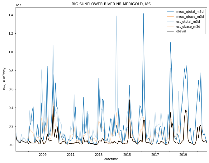
plot data for a site of interest
[23]:
site_no = '07288280'
site_data = combined_obs.loc[combined_obs.site_no == site_no].copy()
site_data.index = site_data.datetime

fig, ax = plt.subplots(figsize=(11, 8.5))
ax = site_data[['meas_qtotal_m3d','meas_qbase_m3d']].plot(ax=ax)
ax = site_data[['est_qtotal_m3d','est_qbase_m3d']].plot(alpha=0.3, ax=ax, color=['C0', 'C1'])
site_data.obsval.plot(ax=ax, c='k')
ax.set_title(meas_metadata.loc[site_no, 'name'])
ax.legend()
ax.set_ylabel('Flow, in m$^3$/day')
[23]:
Text(0, 0.5, 'Flow, in m$^3$/day')
Preprocess head observations
Preprocess head observation data, from the visGWDB program * reproject to the model CRS * cull data to a start_date and optionally, a polygon or set of polygons defining the model area * length units are converted to those of the groundwater model. Open intervals for the wells are converted from depths to elevations * missing open intervals are filled based on well bottom depths (if availabile) and the median open interval length for the dataset. *
Wells are categorized based on the quality of the open interval information (see the documentation for :func:mapgwm.headobs.fill_well_open_intervals). * Prefixes for observation names (with an optional length limit) that identify the location are generated * Similar to with flux observations, assign preliminary observation groups based on geographic areas defined by the * The data DataFrame outputs have the time series; * The metadata DataFrame outputs have site information that
can be input to ``modflow-setup`` to set up the observation input for MODFLOW-6. * Once the model has been run, the observation output from the model can be fed to ``modflow-obs`` along with the data timeseries (below), to set up ``PEST`` observations, or create observation output to be read by ``PEST``.
[24]:
from mapgwm.headobs import preprocess_headobs, get_data

data_file = test_data_path / 'headobs/GW_monthly_stats1990-01-01_2019-12-31.txt'
metadata_file = test_data_path / 'headobs/GW_monthly_meta1990-01-01_2019-12-31.txt'

# output
outputfile = output_folder / 'preprocessed_monthly_headobs.csv'
[25]:
# read the data
data_orig, metadata_orig = get_data(data_file, metadata_file)

# do the preprocessing
data, metadata = preprocess_headobs(data_orig, metadata_orig,
                                    head_data_columns=['head', 'last_head'],
                                    data_length_units='feet',
                                    active_area=delta_extent,
                                    source_crs=4269, dest_crs=5070,
                                    start_date=start_date,
                                    geographic_groups=geographic_groups,
                                    geographic_groups_col='obsgroup',
                                    outfile=outputfile)
starting with 10 unique wells
culling 13 wells with only data prior to start date of 1998-04-01 00:00:00

reading ../mapgwm/tests/data/extents/ms_delta.shp...
--> building dataframe... (may take a while for large shapefiles)
Culling 2 sites outside of the model area defined by ['../mapgwm/tests/data/extents/ms_delta.shp'].
50% of wells (n=4) have incomplete open interval information. Filling screen bottoms with well bottoms where available, and estimating screen tops from median open interval length.
12% of wells (n=1) still missing open interval information; assigned to category 4.

reading ../mapgwm/tests/data/extents/MAP_generalized_regions.shp...
--> building dataframe... (may take a while for large shapefiles)

reading ../mapgwm/tests/data/extents/CompositeHydrographArea.shp...
--> building dataframe... (may take a while for large shapefiles)
writing output/preprocessed_monthly_headobs_info.shp... Done
writing output/preprocessed_monthly_headobs_info.csv
writing output/preprocessed_monthly_headobs.csv
[26]:
data.head()
[26]:
| site_no | datetime | head | last_head | head_std | n | obsprefix | |
|---|---|---|---|---|---|---|---|
| 4 | USGS:332915091025901 | 2003-07-01 | 37.185600 | 37.185600 | NaN | 1 | USGS:332915091025901 |
| 5 | USGS:333411090482201 | 2008-03-01 | 28.096464 | 28.096464 | NaN | 1 | USGS:333411090482201 |
| 6 | USGS:333411090482201 | 2010-03-01 | 27.736800 | 27.736800 | NaN | 1 | USGS:333411090482201 |
| 7 | USGS:333411090482201 | 2015-03-01 | 26.560272 | 26.560272 | NaN | 1 | USGS:333411090482201 |
| 8 | USGS:333411090482201 | 2019-03-01 | 26.484072 | 26.484072 | NaN | 1 | USGS:333411090482201 |
[27]:
metadata.head()
[27]:
| head | head_std | last_head | n | aqfr_cd | nat_aqfr_cd | screen_botm | screen_top | well_depth | well_el | ... | x | y | geometry | well_botm | category | orig_scbot | orig_sctop | obsprefix | group | geo_group | |
|---|---|---|---|---|---|---|---|---|---|---|---|---|---|---|---|---|---|---|---|---|---|
| site_no | |||||||||||||||||||||
| USGS:323340091085201 | 19.50720 | NaN | 19.50720 | 1 | 112MRVA | N100MSRVVL | -88.177600 | -75.985600 | 115.0 | 26.822400 | ... | 452922.427646 | 1.065894e+06 | POINT (452922.4276462687 1065893.772968342) | -88.177600 | 2 | NaN | NaN | USGS:323340091085201 | heads | boeuf |
| USGS:325121091093801 | 29.87040 | NaN | 29.87040 | 1 | 112MRVA | N100MSRVVL | -58.605600 | -46.413600 | 90.0 | 31.394400 | ... | 450055.327781 | 1.098664e+06 | POINT (450055.3277808698 1098664.367787851) | -58.605600 | 2 | NaN | NaN | USGS:325121091093801 | heads | boeuf |
| USGS:332915091025901 | 37.18560 | NaN | 37.18560 | 1 | 112MRVA | N100MSRVVL | 6.705600 | 15.240000 | 108.0 | 39.624000 | ... | 456688.018145 | 1.169617e+06 | POINT (456688.0181453624 1169616.855672613) | -68.376000 | 3 | 6.7056 | 15.24 | USGS:332915091025901 | heads | delta |
| USGS:333411090482201 | 27.60726 | NaN | 27.60726 | 40 | 112MRVA | N100MSRVVL | -81.262968 | -69.070968 | 120.0 | 38.737032 | ... | 478637.876037 | 1.179983e+06 | POINT (478637.8760365412 1179983.321431023) | -81.262968 | 2 | NaN | NaN | USGS:333411090482201 | heads | delta |
| USGS:333633090230701 | 23.77440 | NaN | 23.77440 | 1 | 112MRVA | N100MSRVVL | 3.048000 | 15.240000 | 115.0 | 38.100000 | ... | 517102.401121 | 1.186603e+06 | POINT (517102.4011205511 1186603.416371753) | -76.900000 | 3 | 3.0480 | 15.24 | USGS:333633090230701 | heads | delta_cha |
5 rows × 25 columns
Preprocess ag. water use from the IWUM
read agricultural water use estimates from the Irrigation Water Use Model (IWUM; Wilson, 2020)
cull data to the model area
convert rates from cumulative volumes per time period to cubic meters per day
assign open intervals based on raster surfaces of the estimated production zone for agricultural groundwater use
[28]:
from mapgwm.iwum import preprocess_iwum_pumping

iwum_output = test_data_path / 'iwum/irr_wu_1km_1999_to_2017.nc'
production_zone_top_raster = test_data_path / 'iwum/est_prod_zone_top.tif'
production_zone_botm_raster = test_data_path / 'iwum/est_prod_zone_botm.tif'

outfile = output_folder / 'iwum_m3.csv'
[29]:
ag_wu = preprocess_iwum_pumping(iwum_output,
                                start_date=None,
                                end_date=None,
                                active_area=delta_extent,
                                estimated_production_zone_top=production_zone_top_raster,
                                estimated_production_zone_botm=production_zone_botm_raster,
                                flux_variable='value',
                                nc_crs=5070,
                                nc_length_units='meters',
                                estimated_production_surface_units='meters',
                                model_length_units='meters',
                                outfile=outfile)
reading data from ../mapgwm/tests/data/iwum/est_prod_zone_top.tif...
finished in 0.40s
reading data from ../mapgwm/tests/data/iwum/est_prod_zone_botm.tif...
finished in 0.40s
Reset screen top and bottom to mean elevation at 9 locations where screen top was < screen bottom

reading ../mapgwm/tests/data/extents/ms_delta.shp...
--> building dataframe... (may take a while for large shapefiles)
Culling 14086 sites outside of the model area defined by ['../mapgwm/tests/data/extents/ms_delta.shp'].
wrote output/iwum_m3.csv
[30]:
ag_wu.head()
[30]:
| site_no | x | y | screen_top | screen_botm | start_datetime | end_datetime | q | |
|---|---|---|---|---|---|---|---|---|
| 179 | iwum_179 | 477955.0 | 1041285.0 | 14.093952 | 6.803136 | 2017-06-01 | 2017-06-30 | -2043.222778 |
| 314 | iwum_314 | 476955.0 | 1042285.0 | 13.795248 | 6.400800 | 2017-06-01 | 2017-06-30 | -2093.868652 |
| 315 | iwum_315 | 477955.0 | 1042285.0 | 13.722096 | 6.352032 | 2017-06-01 | 2017-06-30 | -1526.927734 |
| 443 | iwum_443 | 469955.0 | 1043285.0 | 11.457432 | 3.328416 | 2017-06-01 | 2017-06-30 | -1283.890991 |
| 444 | iwum_444 | 470955.0 | 1043285.0 | 11.884152 | 3.947160 | 2017-06-01 | 2017-06-30 | -1245.565308 |
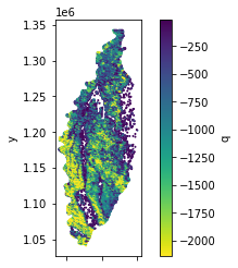
Plot average pumping at each location
[31]:
site_means = ag_wu.groupby('site_no').mean()
ax = site_means.plot(kind='scatter', x='x', y='y', c='q', s=1,
                     cmap='viridis_r', vmin=site_means.q.quantile(0.1))
ax.set_aspect(1)
Preprocess non-ag. water use
Including data from * the USGS Site-Specific Water Use Database (SWUDS) * USGS data on water use for thermo-electric power generation
SWUDs data
SWUDs data are assumed to come in an Excel spreadsheet, that may have incomplete information on well screen intervals
similar to other preprocessing methods, the data are reprojected and optionally culled to an area of interest
if input data do not have information on the well screen intervals, screen tops and bottoms are sampled from raster surfaces bounding estimated production zones; well depth is used to discriminate between zones
data are resampled to continous monthly values between a specified start and end date- typically bracketing the time range that the pumping should be simulated in the model
[32]:
from mapgwm.swuds import preprocess_swuds

swuds_input = test_data_path / 'swuds/withdrawals_test_dataset.xlsx'
worksheet = 'LMG-withdrawals-2000-2018'
outfile = output_folder / 'preprocessed_swuds_data.csv'

dem = test_data_path / 'rasters/dem_mean_elevs.tif'

# raster defining the tops and bottoms of non-agricultural public supply production intervals
# from Knierem
production_zones = {'mrva': (test_data_path / 'swuds/rasters/pz_MRVA_top.tif',
                             test_data_path / 'swuds/rasters/pz_MRVA_bot.tif',
                             ),
                    'mcaq': (test_data_path / 'swuds/rasters/pz_MCAQP_top.tif',
                             test_data_path / 'swuds/rasters/pz_MCAQP_bot.tif',
                             'feet'),
                    'lcaq': (test_data_path / 'swuds/rasters/pz_LCAQP_top.tif',
                             test_data_path / 'swuds/rasters/pz_LCAQP_bot.tif')
                    }
[33]:
swuds_results = preprocess_swuds(swuds_input, worksheet,
                                 dem=dem, dem_units='feet',
                                 start_date=None,
                                 end_date=None,
                                 active_area=test_data_path / 'extents/ms_delta.shp',
                                 production_zones=production_zones,
                                 source_crs=4269,
                                 dest_crs=5070,
                                 data_length_units='feet',
                                 data_volume_units='mgal',
                                 model_length_units='meters',
                                 outfile=outfile)
reading ../mapgwm/tests/data/extents/ms_delta.shp...
--> building dataframe... (may take a while for large shapefiles)
Culling 831 sites outside of the model area defined by ['../mapgwm/tests/data/extents/ms_delta.shp'].
reading data from ../mapgwm/tests/data/rasters/dem_mean_elevs.tif...
finished in 0.26s
reading data from ../mapgwm/tests/data/swuds/rasters/pz_MRVA_top.tif...
finished in 0.01s
reading data from ../mapgwm/tests/data/swuds/rasters/pz_MRVA_bot.tif...
finished in 0.01s
reading data from ../mapgwm/tests/data/swuds/rasters/pz_MCAQP_top.tif...
finished in 0.01s
reading data from ../mapgwm/tests/data/swuds/rasters/pz_MCAQP_bot.tif...
finished in 0.01s
reading data from ../mapgwm/tests/data/swuds/rasters/pz_LCAQP_top.tif...
finished in 0.01s
reading data from ../mapgwm/tests/data/swuds/rasters/pz_LCAQP_bot.tif...
finished in 0.01s
processed SWUDS data written to output/preprocessed_swuds_data.csv and in dataframe attribute
writing output/preprocessed_swuds_data.shp... Done
A mapgwm.swuds.Swuds object is returned, which has a dataframe attribute:
[34]:
swuds_results.df.head()
[34]:
| site_no | q | q_monthly | month | well_elev | depth | screen_bot | screen_top | x | y | start_datetime | geometry | |
|---|---|---|---|---|---|---|---|---|---|---|---|---|
| 2010-01-01 | 322431090530201 | 20895.471597 | 5.52 | JAN_VAL | 85.0 | 37.1856 | 47.8144 | 67.8144 | 478430.626345 | 1.050261e+06 | 2010-01-01 | POINT (478430.6263445358 1050260.766381889) |
| 2010-02-01 | 322431090530201 | 20895.471597 | 5.52 | FEB_VAL | 85.0 | 37.1856 | 47.8144 | 67.8144 | 478430.626345 | 1.050261e+06 | 2010-02-01 | POINT (478430.6263445358 1050260.766381889) |
| 2010-03-01 | 322431090530201 | 20895.471597 | 5.52 | MAR_VAL | 85.0 | 37.1856 | 47.8144 | 67.8144 | 478430.626345 | 1.050261e+06 | 2010-03-01 | POINT (478430.6263445358 1050260.766381889) |
| 2010-04-01 | 322431090530201 | 20895.471597 | 5.52 | APR_VAL | 85.0 | 37.1856 | 47.8144 | 67.8144 | 478430.626345 | 1.050261e+06 | 2010-04-01 | POINT (478430.6263445358 1050260.766381889) |
| 2010-05-01 | 322431090530201 | 20895.471597 | 5.52 | MAY_VAL | 85.0 | 37.1856 | 47.8144 | 67.8144 | 478430.626345 | 1.050261e+06 | 2010-05-01 | POINT (478430.6263445358 1050260.766381889) |
Water use for thermoelectric power generation
similar to the SWUDs data, data for water use related to TE power generation are assumed to come in a spreadsheet
however, the column names might different between different datasets.
therefore, the first step is to read in the data using a function that harmonizes the column names, and then combine the data using
DataFrame.append():
[35]:
from mapgwm.te_wateruse import read_te_water_use_spreadsheet, preprocess_te_wateruse

df2010 = read_te_water_use_spreadsheet(test_data_path / 'swuds/2010_Thermo_Model_Estimates.xlsx',
                                       date='2010',
                                       x_coord_col='Longitude, decimal degrees',
                                       y_coord_col='Latitude, decimal degrees',
                                       q_col='USGS-Estimated Annual Withdrawal (Mgal/d)',
                                       site_no_col='PLANT CODE',
                                       site_name_col='PLANT NAME',
                                       source_name_col='NAME OF WATER SOURCE',
                                       source_code_col='USGS WATER SOURCE CODE',
                                       sheet_name='Report_table_UPDATED', skiprows=2)

df2015 = read_te_water_use_spreadsheet(test_data_path / 'swuds/2015_TE_Model_Estimates_lat.long_COMIDs.xlsx',
                                   date='2015',
                                   x_coord_col='LONGITUDE',
                                   y_coord_col='LATITUDE',
                                   q_col='WITHDRAWAL',
                                   site_no_col='EIA_PLANT_ID',
                                   site_name_col='PLANT_NAME',
                                   source_name_col='NAME_OF_WATER_SOURCE',
                                   source_code_col='WATER_SOURCE_CODE',
                                   sheet_name='2015_ANNUAL_WD_CU', skiprows=0)
df = df2010.append(df2015)
We can then run the data through a similar function to that used for SWUDs:
[36]:
outfile = output_folder / 'preprocessed_te_data.csv'

estimated_production_zone_top = test_data_path / 'swuds/rasters/pz_MCAQP_top.tif'
estimated_production_zone_botm = test_data_path / 'swuds/rasters/pz_MCAQP_bot.tif'

te_results = preprocess_te_wateruse(df, #dem=dem, dem_units='feet',
                                    start_date='2008-01-01',
                                    end_date='2017-12-31',
                                    active_area=test_data_path /'extents/ms_delta.shp',
                                    estimated_production_zone_top=estimated_production_zone_top,
                                    estimated_production_zone_botm=estimated_production_zone_botm,
                                    estimated_production_surface_units='feet',
                                    source_crs=4269,
                                    dest_crs=5070,
                                    data_volume_units='mgal',
                                    model_length_units='meters',
                                    outfile=outfile)
reading ../mapgwm/tests/data/extents/ms_delta.shp...
--> building dataframe... (may take a while for large shapefiles)
Culling 405 sites outside of the model area defined by ['../mapgwm/tests/data/extents/ms_delta.shp'].
reading data from ../mapgwm/tests/data/swuds/rasters/pz_MCAQP_top.tif...
finished in 0.17s
reading data from ../mapgwm/tests/data/swuds/rasters/pz_MCAQP_bot.tif...
finished in 0.16s
wrote output/preprocessed_te_data.csv
writing output/preprocessed_te_data.shp... Done
[37]:
te_results.head()
[37]:
| site_no | start_datetime | x | y | screen_top | screen_botm | q | geometry | source_name | site_name | |
|---|---|---|---|---|---|---|---|---|---|---|
| 2008-01-01 | 2059 | 2008-01-01 | 497139.150871 | 1.249816e+06 | -147.409514 | -162.649514 | 0.0 | POINT (497139.1508711056 1249816.468462982) | Wells | L L Wilkins |
| 2008-02-01 | 2059 | 2008-02-01 | 497139.150871 | 1.249816e+06 | -147.409514 | -162.649514 | 0.0 | POINT (497139.1508711056 1249816.468462982) | Wells | L L Wilkins |
| 2008-03-01 | 2059 | 2008-03-01 | 497139.150871 | 1.249816e+06 | -147.409514 | -162.649514 | 0.0 | POINT (497139.1508711056 1249816.468462982) | Wells | L L Wilkins |
| 2008-04-01 | 2059 | 2008-04-01 | 497139.150871 | 1.249816e+06 | -147.409514 | -162.649514 | 0.0 | POINT (497139.1508711056 1249816.468462982) | Wells | L L Wilkins |
| 2008-05-01 | 2059 | 2008-05-01 | 497139.150871 | 1.249816e+06 | -147.409514 | -162.649514 | 0.0 | POINT (497139.1508711056 1249816.468462982) | Wells | L L Wilkins |
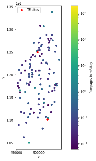
Plot the locations of SWUDs and TE water use
[38]:
fig, ax = plt.subplots(figsize=(11, 8.5))
ax = swuds_results.df.plot.scatter(x='x', y='y', c='q_monthly',
                                   cmap='viridis',
                                   vmax=swuds_results.df.q.quantile(0.9),
                                   norm=mpl.colors.LogNorm(), ax=ax)
te_results.plot.scatter(x='x', y='y', c='r', ax=ax, label='TE sites')
ax.legend()
ax.set_aspect(1)
cax = fig.get_axes()[1]
#and we can modify it, i.e.:
cax.set_ylabel('Pumpage, in m$^3$/day')
[38]:
Text(0, 0.5, 'Pumpage, in m$^3$/day')
